Quick facts
- Prototype: physis, Apache 2.0, github.com/kuberoot-dev/physis
- Core objects: Problem, Substrate, Receipt, Mandate and Link; no Node objects
- Physics modeled: 18; CPU and an Apple M4 GPU on real hardware, 16 emulated
- Main result (Q3 2026): Energy −90% and carbon −91% against “Kubernetes today”; −84% carbon even at the pessimistic end of every assumption
- Conformance: 17/17 tests on five testbeds, including a four-node cluster on Hetzner servers and a node with no container runtime
- Built on: kuberoot (Kubernetes 1.37), Cozystack workshop cluster
Source: github.com/kuberoot-dev/physis, results/ and docs/verification.md
Infrastructure is almost always built for yesterday’s problems. Unix was designed for time-sharing machines, TCP/IP for a network that had to survive the loss of nodes, and Borg for a single company with its own data centers, where hardware heterogeneity was mostly hidden behind a uniform resource model. Kubernetes inherited from Borg nearly everything that lies deeper than its API. Each of these systems was a brilliant answer to its own questions, and each was then stretched for decades over questions its authors never even asked. In other words, today’s problems are being solved by a convention the industry settled on, one that was never designed to solve them.
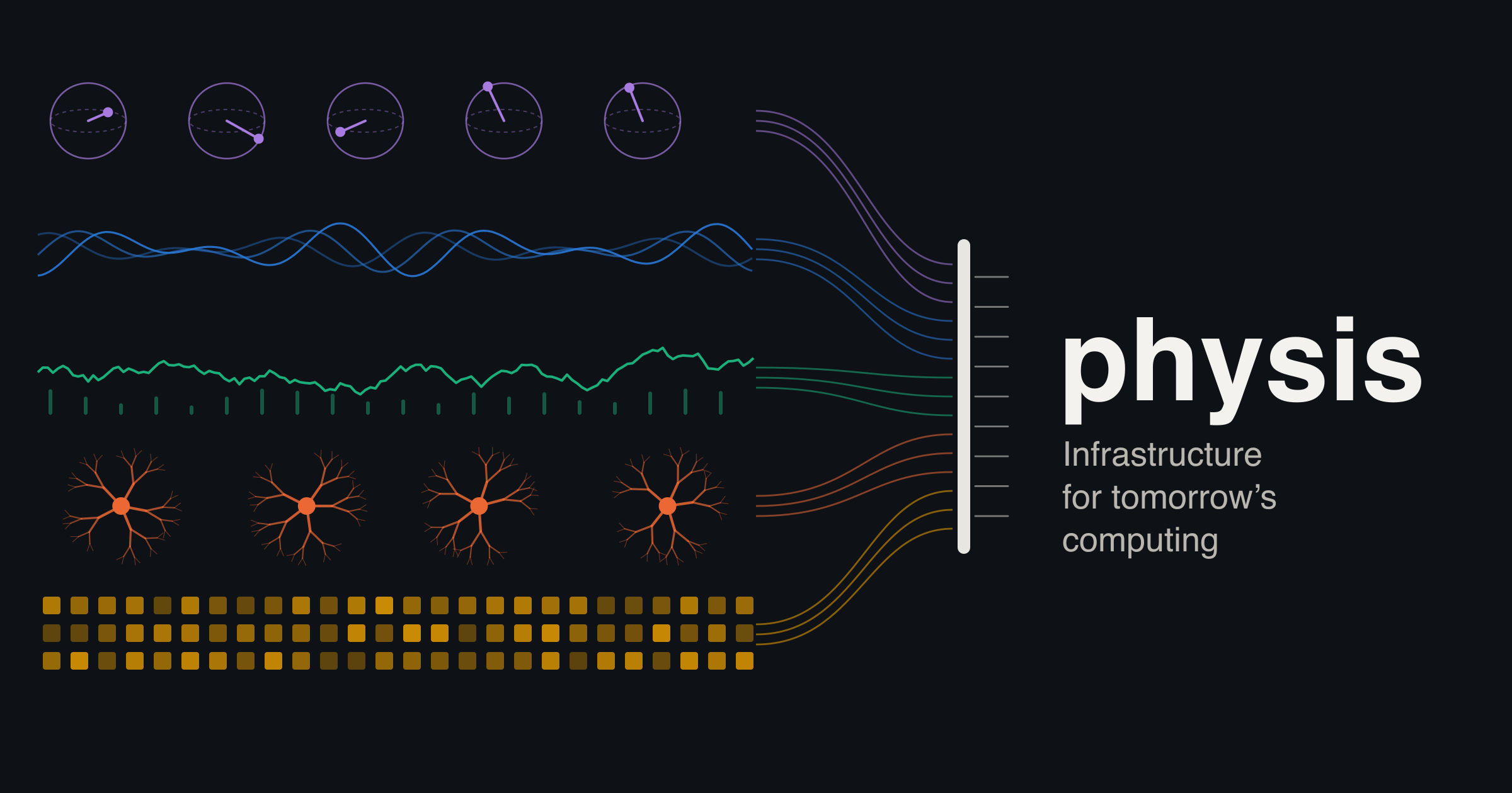
Quantum, photonic, analog, living and silicon compute converging under a single scheduling layer
In this article we approach the problem from the other end. First we work out which problems will be solved tomorrow and what the physics of computation, the economics and the requirements for trust will look like. Only then do we derive the corresponding infrastructure layer from that and build a prototype that chooses not only the place and time for a problem, but also the physics of the computation itself, from a CPU to a quantum computer to living neurons.
I have approached this topic more than once before; once, together with colleagues, we even made a public attempt to discuss it in an episode of the Kuber Community Podcast. Since then I kept quietly digging through papers and research on the subject (not understanding all of it, of course) and forming my own picture of what awaits us tomorrow.
You might say: old man, take your pills, why do you even need this? But I work on the team that builds the Cozystack platform, and I would like Cozystack to be not just a solution for today’s problems, but to stay relevant and fresh for a couple of decades. For that, we need to start thinking about the future now.
The late Gennady Konstantinov of HSE University said, either on the make sense podcast or in a talk at one of the ProductSense conferences, that in a world of rapid change, long-term strategic planning becomes a far more important activity than in a world where change is relatively slow. At first glance the idea is counterintuitive, but he offered a simple metaphor: the faster your car is moving, the farther ahead you need to look. Personally, I found that image convincing.
There will be many links to primary sources. They are dry and difficult, but this is the way.
The article is long, so here is its outline:
- How we will compute tomorrow — the trends that are already visible, from the energy ceiling to computing on neurons in a dish.
- The economics of the day after tomorrow — where money in IT is going and what that means for infrastructure.
- People, agents and trust — what the Institute for the Future and the Future Today Strategy Group forecast, and how that maps onto infrastructure.
- Principles derived from these trends.
- An audit of Kubernetes: what it gets right from the standpoint of our problem, and what was built for yesterday’s world.
- The design of a new layer: no concept of a node, a scheduler that chooses physics, a network where a participant is found not by IP address but by a cryptographically verifiable identity, and the cloud as a market of substrates, that is, of any hardware on which computation runs.
- The physis prototype running on eighteen different physics of computation, two of them on real hardware.
- How we tested physis and what came out of it.
- Conformance for systems of tomorrow — a test suite that any implementation can pass (we designed it ourselves).
- Limitations — where we might be wrong.
- What comes next.
- Unsolicited advice for the CNCF: how to evolve Kubernetes now so that it suits both yesterday’s and tomorrow’s world, what to keep in the core and what to make pluggable.
- Cozystack 3.0 as a platform for the infrastructure layer of tomorrow.
The code, data and tests are open under the Apache 2.0 license. I would be grateful for feedback.
1. How we will compute tomorrow
Roy Amara, president of the Institute for the Future, formulated the law that bears his name: we overestimate the effect of a technology in the short run and underestimate it in the long run [1]. So what follows is not about forecasts, but about trends that already have measurable manifestations. Each of them we will later turn into a requirement for infrastructure.
F1. Energy becomes the main constraint
In 2026, Amazon, Microsoft, Alphabet and Meta together are spending on the order of $720–740 billion on infrastructure [2]. Gartner forecasts worldwide IT spending in 2026 at $6.37 trillion, up 14.2% year over year [3]. Yet the bottleneck turned out to be not chips but the plain electrical grid. Connecting a large data center to the grid takes years in a number of regions; the capacity price at PJM, the largest grid operator in the eastern United States, rose from $29 to $330 per megawatt-day over two auctions; gas turbines have multi-year waiting lists; and the largest cloud companies (the hyperscalers) are signing contracts with nuclear power plants [4].
Energy also has a flip side that is usually forgotten. All the energy a computer consumes becomes heat, so computation, strictly speaking, turns electricity into heat and along the way gives us some answers to the questions we asked. There is a physical minimum, the Landauer limit, which is the energy required to erase one bit [5], and modern chips spend orders of magnitude more. But in the limit, computation runs up not against the energy going in, but against the ability to remove heat. Hence water for cooling, cryogenics for quantum and superconducting machines, and interest in reversible computing, which recovers part of the energy.
There are also constraints that get discussed less often. In 2024, large power transformers had an average lead time of 120 weeks, compared with 50 weeks in 2021 [6], and gas turbines have multi-year waits [4]. Helium is needed for the cryogenics of quantum machines and superconducting logic. Oxygen, on the other hand, will not become a constraint (this was a revelation for me): all the fossil fuel burned worldwide, together with every other oxygen-consuming process, reduces the amount of this gas in the atmosphere by roughly 19 molecules per million per year, or 0.002% [7], and data centers account for only a small share of that.
What this means for infrastructure. Energy stops being a simple line item in accounting reports and bills and becomes a strategic resource, planned the same way CPU cores are planned today, and carbon, the price per hour and heat are considered together with it.
F2. The physics of computation diverges
Until recently, heterogeneous hardware meant CPUs and GPUs from different vendors. Today there are machines that compute in fundamentally different ways:
| Physics | What it is | Where we are now |
|---|---|---|
| Analog in-memory computing | Matrix multiplication with currents directly in memory cells, without moving data around | The IBM HERMES chip on phase-change memory: 63.1 TOPS at 9.76 TOPS/W, effective precision of 3–4 bits [8] |
| Neuromorphic chips | No clock; computation proceeds through spike events | Hala Point at Sandia: 1152 Loihi 2 chips, 1.15 billion neurons [9]; the first Loihi used about 20–25 pJ per synaptic operation [10] |
| Probabilistic computers on p-bits | The chip produces samples from a distribution, using thermal noise as a resource | A stochastic magnetic tunnel junction — an estimated 2 fJ or so per random bit [11]; the first Extropic devices are with early users [12] |
| Ising machines | An optimization problem is encoded into a physical system, which settles into its energy minimum on its own | An FPGA using simulated bifurcation solved MaxCut on 2000 vertices 124 times faster than an optimized simulated annealing method [13]; optical machines operate at room temperature [14] |
| Reversible computing | Logic recovers part of the switching energy | The Vaire test chip — about 30% energy savings on the same task [15] |
| Superconducting logic | Switching at almost no energy, but at 4 K | imec promises a data center the size of a shoebox [16]; cooling at 4 K costs at least 74 W per watt of removed heat by the Carnot limit, under 400 W/W for the best installations [17], about 740 W/W for ordinary Collins- and Brayton-cycle installations, and 5–7.5 kW/W for small cryocoolers [18] |
| Photonic computing | Multiplication with light | 0.27 pJ per multiply-accumulate for the laser alone in a laboratory processor [19] |
| Quantum processors | Integrated into supercomputing centers under a conventional scheduler | The PCSS center in Poznań under Slurm [20]; Google’s superconducting Sycamore setup, including cryogenics, drew up to 26 kW [21] |
| Living neurons | Cultures of human neurons as a computer | Cortical Labs CL1 — neurons grown from human stem cells on a silicon chip; sells for about $35 thousand, draws about 20 W, and the neurons live up to six months [22]; FinalSpark organoids live about 100 days [23] |
| Trainable physics and computing materials | Sound, light and mechanics are trained like a neural network; a metamaterial works as logic | Physical neural networks [24]; a mechanical metamaterial with reconfigurable logic [25] |
Alongside the exotic, there is a wave of far more down-to-earth architectures. They change not the physics of switching but the way computation is done: where it happens, how numbers are represented and what precision is actually needed. These are the ones that will land in data centers in the coming years.
| Architecture | What changes | What is known |
|---|---|---|
| Systolic tensor arrays | Matrix multiplication as a wave through a grid of multipliers; data is reused without memory accesses | TPU v1: 65,536 eight-bit multipliers, 92 TOPS, 40 W under load, 30–80 times higher TOPS/W than GPUs and CPUs of its time [26]; TPU v4 — another 2.7 times better performance per watt [27] |
| Dataflow and spatial processors | No caches or arbiters: the compiler statically lays out the dataflow across the die, and timing is deterministic | Groq TSP: about 750 TOPS int8 and 220 MiB of on-die SRAM [28]; Cerebras WSE-3 is an entire wafer: 900 thousand cores and 44 GB of SRAM [29]; SambaNova SN40L fuses a model’s operators into a single pipeline [30] |
| Processing in DRAM | Compute units sit in the memory banks; data does not travel to the processor | Samsung HBM-PIM: 1.2 TFLOPS from HBM2 banks [31], with 3.5 times lower energy per transferred bit [32]; UPMEM — production modules, on average 28–93 times faster than a CPU on 13 of 16 PrIM benchmarks [33] |
| Reduced and block precision | Precision becomes a parameter: FP8, and in Microscaling formats a block of 32 numbers shares one scale | FP8 preserves the quality of 16-bit training on models up to 175 billion parameters [34]; training with MXFP4 weights costs only a small loss of accuracy [35]; eight-bit integer multiplication is roughly 18 times cheaper than 32-bit floating point [36] |
| Stochastic computing | A number is the fraction of ones in a random bit stream; multiplication is a single logic gate | Precision grows as the logarithm of the stream length, but the circuit is tiny and tolerates bit errors [37] |
| Hyperdimensional computing | Computation over random vectors with thousands of dimensions: binding, bundling, comparison | Robust to failures of individual bits [38]; in phase-change memory, more than 6 times less energy than a digital implementation [39] |
| CGRAs and FPGAs | A grid of compute units reconfigured for the task instead of an instruction stream | Most CGRAs perform more operations per watt than GPUs, some by two orders of magnitude [40] |
For the control layer, this wave matters more than the exotic machines. Here the quality-versus-energy trade-off becomes routine. The same model in FP4 is cheaper than in FP8 but slightly less accurate, and whether that is good enough should be decided by the problem itself, not by the programmer.
Each of these physics has its own speed, precision, noise, calibration and cost per operation. Heterogeneity here means not “different vendors of the same principle” but different ways of computing.
New physics also breaks familiar operational assumptions. The state of an analog array, a trained metamaterial or a living culture cannot be “snapshotted” and moved to another machine, so migration comes down to retraining on a new medium. That means the true state must live outside the hardware, in the description and the training data, and the hardware becomes a reproducible execution. Operations turn into caring for an organism: calibration, retraining, aging, cryogenics and, for organoids, literal feeding. And living hardware brings ethics. This is the first infrastructure in which a resource may have rights, so the platform needs usage policies, not just RBAC.
What this means for infrastructure. A resource can no longer be described in cores and gigabytes. It has to be described by its physics: the operation, speed, energy per operation, precision, noise, calibration windows and capacity. And the scheduler must choose the physics the same way it chooses a location.
F3. The boundaries of the machine and the node blur
CXL makes it possible to pool memory and already offers a memory domain spanning the whole data center over optics; a review in Nature Reviews Electrical Engineering explicitly calls this a “data center as a single chip” design [41]. NVIDIA announced Vera Rubin Ultra with 576 GPUs connected by a single NVLink switching fabric [42], and Oxide designs a rack rather than a server [43]. The “node” as an indivisible server with a CPU, memory and disks matches the way modern hardware is built less and less.
F4. Agents become the main users
Agents are given an isolated sandbox for each session, a lightweight virtual machine (microVM) [44]. Machine-to-machine payment protocols (x402, contributed to the Linux Foundation, and AP2, contributed to FIDO) let an agent pay another agent under a human’s mandate, that is, a human-signed authorization stating how much the agent may spend, where and until when [45, 46]. Amy Webb of the Future Today Strategy Group calls this the “next internet,” built for agents [47]. The main caller of the APIs of tomorrow’s infrastructure will be a machine making thousands of calls per second.
F5. Trust stops being free
In its forecast for 2036, the Institute for the Future highlights three themes about knowledge and trust [48]: “discernment,” meaning whatever replaces the “seeing is believing” heuristic; a crisis of scientific knowledge, in which generative systems produce plausible results and fake citations on demand; and the “four cultures of AI.” A year earlier, IFTF wrote separately about a crisis of proving one is human [1]. The technical response is already being built: hardware attestation, computation over encrypted data moving onto specialized accelerators (FPGAs for now, ASICs in development) [49], and formal verification in Lean at AWS [50]. Trust becomes not an emotion or a feeling but a rigorous data structure that can be verified.
F6. Compute becomes a commodity
The price of reaching a fixed level of language model answer quality falls by a median of roughly 50 times per year, ranging from 9 to 900 times depending on the task [51]. History suggests, however, that total spending will not fall but grow. This is the Jevons paradox [52]: a resource that gets cheaper gets consumed more and more. The CME, ICE and Nodal exchanges are preparing futures on GPU-hours [53]. Per-seat pricing for cloud software (SaaS) is giving way to pricing by outcome [54]. Starting January 12, 2027, the EU Data Act prohibits charging for switching cloud providers, including data egress fees when moving [55]. Compute is becoming increasingly dependent on energy prices and depreciation, and what retains customers is price, quality and trust rather than vendor lock-in. At Berkeley this logic has been taken all the way to the “sky computing” architecture, in which the user hands a job to a broker that chooses the cloud itself based on price and availability [56].
F7. Compute moves where there is no constant connectivity
Physical AI, robots and world models live in a closed loop of “data collection — training — deployment on edge devices — fine-tuning” [57]. IFTF names the shift “from large language models to large world models” one of the forces of the decade [48]. Data centers are being designed even in orbit. In Project Suncatcher, Google together with Planet Labs plans to launch two prototype satellites with TPUs by early 2027, and Starcloud has already put a satellite with an NVIDIA GPU into orbit [58]. Connectivity there is intermittent, and for such environments the IETF standardized a store-and-forward protocol, Bundle Protocol v7 [59]. A control center that must always be reachable does not work there.
F8. Systems start being designed by machines
At Berkeley, a “generate — evaluate — refine” loop found algorithms better than human-designed ones for a range of systems problems (scheduling across cloud regions, load balancing across “experts” in mixture-of-experts (MoE) models, transaction scheduling), running up to 5 times faster or costing up to 50% less [60]. The bottleneck of this approach turns out to be an accurate evaluator. So infrastructure needs a built-in digital twin, that is, a simulator that reproduces the behavior of the real system, along with specifications against which a machine can check its own changes.
F9. State matters more than computation
Durable execution, an approach in which every step of a program is recorded so that after a failure it resumes from the same point, makes program state primary and computation an executor that can be restored; the DBOS project began as research into “an OS whose entire state is stored in database tables” [61]. Hydro and the CALM theorem show which distributed programs can do without coordination [62, 63], while Ink & Switch’s research on local-first software, where data lives primarily on the user’s device, and on “malleable” software that users can reshape for themselves, returns data to its owner [64, 65]. The executor becomes replaceable, and value shifts to data and its provenance.
F10. Uncertainty becomes the norm
Probabilistic chips produce samples, analog ones produce an approximate result with noise, quantum ones produce a distribution of outcomes over many repeated measurements, and AI models produce an answer with a confidence level. The correct answer is being replaced by an answer that is good enough with a known probability. A system that only knows “desired state: three replicas” has nothing to say about such a world.
From the practical to the insane
If we sort all of this by maturity, we get the following ladder:
| Maturity | What | Why it matters for the layer |
|---|---|---|
| Already in production | CXL memory pools, optical switching fabrics, microVMs for agents, durable execution, shifting jobs to hours with cleaner electricity | The node stops being the unit; work must survive the failure of its executor |
| The next few years | AI that designs systems; provable code; languages for the whole cloud; brokers across clouds; intent instead of commands | Twins, specifications and a plan before execution are needed |
| Different physics | Analog, neuromorphic, probabilistic, photonic, reversible and superconducting machines; quantum processors in the data center | The scheduler must choose the physics |
| Insane, but funded | Data centers in orbit, DNA storage in a rack [66], living neurons as a computer | Intermittent connectivity, limited hardware lifetime, ethics of the resource |
2. The economics of the day after tomorrow
IT is in a record money boom, and debt is growing alongside it. Morgan Stanley estimates that the debt of AI companies will exceed $500 billion in 2026 [67], and the Bank of England warns of a maturity mismatch: the life cycle of AI chips is short and uncertain, while lenders prefer to lend over longer terms [68]. If revenue does not catch up with investment, the world will get what it already saw with fiber in 2001, when investors went bankrupt and the surplus infrastructure passed to the next generation at scrap prices. If revenue does catch up, compute becomes a utility, cheap per unit and enormous in volume. And if energy turns out to be the main constraint, compute will be tied to the places where energy is available, and its price will be counted in joules.
Under any of these three outcomes, the same things reshape infrastructure:
- The unit of value shifts from the per-seat SaaS license to the action, the outcome, the token, and eventually the joule.
- Compute gets a market price, which means accounting standards and provable delivery are needed.
- The buyer is a machine that pays for each call within a budget and a mandate.
- Hardware has a short economic life, buildings a long one. Five generations of accelerators plus exotic hardware will sit in one pool, and the winner is whoever can squeeze money out of old hardware.
- Energy is the largest cost item and a new source of revenue. Work that can be deferred is paid for by the grid itself.
- Moving away from a provider gets cheaper, and lock-in stops being a business model.
- Labor gets cheaper. AI writes code and operates systems, so the platform has to be operable by agents.
This leads to what we consider the most counterintuitive idea of this section. The main economic opportunity of the coming years is not to build new capacity, but to cheaply assemble into working clouds what has already been built during the bubble: used GPUs, underutilized data centers, nighttime energy, the hardware of small providers. The layer that turns this heterogeneous fleet into a sovereign, measurable and verifiable cloud is needed under any outcome, whether a soft landing or a correction.
The other side of the energy bill is made up of heat, water and carbon. The layer has to account not only for the joules going in, but also for where the heat goes. In Stockholm, data centers already sell it to the district heating network [69]. It also has to account for how much water went into cooling and how much CO₂ stands behind a given joule at a given hour in a given place. The scheduler then decides not “where is electricity cheapest” but “where did this joule arrive most cheaply and leave most usefully.”
If compute becomes a commodity and leaving a supplier is free, then everyone works on a single interface, and companies compete on how they package it. This has already happened with electricity and the standard outlet, with the S3 API, and with OpenAI-compatible interfaces for serving models. A standard does not remove competition from technology; it pushes it down, into the cost of the joule, and up, into the product on top of the standard: domain, trust, convenience, guarantees. But the “single interface” model has its limits. A standard always remains the lowest common denominator. It covers what everyone agrees on, that is, yesterday, while everything new first appears as a specific vendor’s extension. Vendors bring lock-in back through extensions, following the old “embrace, extend, extinguish” recipe. S3 is standard, for example, but it is surrounded by hundreds of services coupled to it. Lock-in moves from technology into data gravity (petabytes of data take a long time to move, even if the ability to move them costs nothing), into contracts and volume discounts, into the team’s skills, and into integration with identity and audit systems. Whoever owns the standard owns the market. By opening Kubernetes, Google made portable the layer on which lock-in to the market leader rested, which is a variant of Joel Spolsky’s “commoditize your complements” strategy [70].
The main risk of such a world is that the interface gets captured by someone who sits on top of it and starts extracting rent. That is why the standard must belong to a neutral foundation and be verified by open conformance tests.
A market with four roles forms around the single interface:
| Role | Who | What they compete on |
|---|---|---|
| Substrate providers | Owners of hardware of any physics, data centers, energy, spare capacity | Cost per joule, location, reliability |
| Method providers | Models, solvers, compilers that translate a problem into a form for a specific physics, algorithms | Quality per joule |
| Product providers | Those who assemble methods and substrates into an outcome for the customer: a sovereign cloud for a bank, a GPU cloud for SaaS, AI for a clinic | Domain, trust, convenience, pricing structure, guarantees — in essence, insurance of the outcome |
| Consumers | People and, increasingly, agents | An agent compares providers automatically and instantly, so the market becomes very efficient |
To keep the market from turning into an app store with a 30% commission, four conditions are needed: the standard held by a neutral foundation, open conformance, portable settlement and reputation, and no mandatory intermediary between consumer and provider.
3. People, agents and trust
The Institute for the Future has been publishing a ten-year forecast for several decades [1]. Its edition “2036 — What We Choose Next” (October 2026) consists of ten forecasts in three blocks [48]:
- Trust and knowledge: discernment in a world where seeing is no longer believing; the future of scientific knowledge; the “four cultures of AI” (without AI, augmented by AI, alongside AI, and governed by AI).
- Where power and capital migrate: the “Muddle Powers,” for which energy rather than ideology sets the agenda; “China Is Everywhere”; the world after financialization; the end of the insurance bargain.
- The fabric of everyday life: loneliness, which may become the defining social force of the decade; life in extreme heat, where warming of 1.5 °C above pre-industrial levels (the limit set by the Paris Agreement) becomes not a ceiling but a starting point; the transition from language models to world models.
A year earlier, in its 2025–2035 edition “Strategy in the Age of Chaos,” IFTF started from the premise that the operating systems of society (money, knowledge, climate, education and even childbirth) are becoming unrecognizable [1]. Its themes include technology as a new religion, AI as a public good on the utility model (Public Option AI), “post-epistemological truth,” the gamblification of markets that appear and vanish as in a casino, life in a world where warming has already exceeded 1.5 °C, the Paris Agreement limit, algorithmic harm as a business model, a “backup of civilization on the Moon,” and a crisis of proving that you are human. Two threads matter here for infrastructure: AI and compute as a public good (an argument for an open standard layer not owned by a single vendor) and trust that has to be rebuilt from scratch.
In 2026, Amy Webb’s Future Today Strategy Group announced the “creative destruction” of its classic trends report and presented the Convergence Outlook on converging technologies [47]. The convergences include “living intelligence” (AI, sensors and biotech) and “limitless labor” (agents, robots and automated factories), and separately Webb talks about the “next internet,” which is being built for agents.
Two conclusions follow for infrastructure.
Where the human ends and the agent begins. The human should set what they are accountable for, that is, values, limits and the mandate. Translating that into parameters is the agent’s job. A human should not be entering “accuracy 0.97 and 4096 samples”; they answer the questions “how confident must the answer be, how much am I willing to pay, by what deadline, what must not be put at risk.” Work should stop and wait for a human signature not at every step, but where a mistake would be expensive: when an action is hard to undo, when it costs a lot of money, or when its consequences affect many people and systems. The more of these three signs coincide, the earlier the system should stop and ask a human how to proceed. This determines how the system is built. Its core is designed for programs that call the API, and on top of the same core people get familiar tools: a console, reports and monitoring dashboards. The code assumes that the caller may be wrong or malicious. A human presses a button once a minute, while an agent makes a thousand calls per second and persistently looks for workarounds. So before every action, the server itself checks whether it can be performed: whether the budget is sufficient, whether the zone and jurisdiction are permitted, whether it violates rules that must always hold. This is done on the server precisely because an agent will simply bypass a button in the UI. Every action either executes completely or not at all, with no half-finished intermediate states, and before it runs it has a plan and a cost estimate. Some actions require a human signature, verified cryptographically rather than by the presence of a button in the interface. And the “four cultures of AI” become autonomy levels, that is, a setting rather than separate products (the prototype has three; working entirely without AI stays outside the system).
Trust as a data structure. Every result should come with a receipt recording who asked and under what mandate, what was computed, on what, from which data, with what confidence and at what cost. Receipts are signed and chained, and anyone can verify them without access to the system. IFTF’s forecast about “discernment” then becomes a property of infrastructure, and trust is verified rather than judged by eye.
Verification also costs energy, so its depth is chosen according to the stakes, from cheap to expensive:
- Signatures and provenance — for everything.
- Hardware attestation — proof that the computation ran on exactly the claimed device in the claimed location.
- Cross-checking on a different physics or with a different provider.
- A statistical certificate for probabilistic computation, which provides confidence rather than “correctness.”
- A formal proof — for critical code and policies, as with Cedar at AWS [50].
The depth of verification, from a receipt for a routine problem to a formal proof for a payment core, becomes one more quantity in the same cost model, alongside time, energy and money.
The receipts themselves are best written to an append-only log, where entries can only be added, never changed or deleted, and which anyone outside can verify, following the model of Certificate Transparency [71, 72] or Sigstore’s Rekor log [73]. Then history cannot be forged retroactively, not only within a single agent’s chain but across the whole system.
4. Principles
Fourteen principles follow from the ten forces. They also became the basis of the conformance suite.
| # | Principle | From which forces |
|---|---|---|
| P1 | The interface is preserved; everything beneath it is replaceable. The Kubernetes API is the language of today; those who demand a new language lose | F6; the history of Plan 9 and Lisp machines |
| P2 | A request is an outcome, not resources. Quality, deadline, budget, permitted locations; choosing the algorithm, physics, place and time is the system’s job | F2, F4, F6, F10 |
| P3 | Physics is described explicitly, and every number has a provenance | F2, F3 |
| P4 | Cost is a mandatory part of the description. Every problem and every plan states time, energy, carbon and money, and it is visible why one option beats another | F1, F6 |
| P5 | Uncertainty is part of the system’s promise. Quality as a probability with a lower bound; do not promise what has not been measured; plan by forecast, evaluate by fact | F10, F5 |
| P6 | Closed loop. Runs train the models; a digital twin tests the policies | F8, F2 |
| P7 | No nodes. Substrates pull work themselves; a failure is work that was not picked up | F3, F7 |
| P8 | Local autonomy. Work that has started is carried to completion without the global level | F7 |
| P9 | Verifiability of the result. Signature, chain, verification without access to the system | F5 |
| P10 | People set the limits, agents act within them: a signed mandate, autonomy levels | F4, F5 |
| P11 | Data and compute have a location and a jurisdiction; sovereignty is a hard constraint | F5, F6 |
| P12 | Flexible work follows clean and cheap energy; urgent work is not delayed | F1 |
| P13 | An open standard, verified by tests | F6 |
| P14 | The agent is the API’s first user: strict schemas, a plan before execution, cost before launch | F4 |
5. Auditing Kubernetes
Kubernetes grew out of Borg [74], one company’s system for long-running services and batch jobs on CPUs. Borg mostly hid machine heterogeneity behind a uniform resource model, and it leaked into the API only as machine attributes in placement constraints. Much of it is right and will stay.
What is right and stays
- Declarative API and reconciliation. A resource describes intent, and a controller drives the world toward it. This technique will outlive any physics.
- API extensibility: CRDs, API aggregation, change subscriptions (list/watch), RBAC, admission-time object checks. This is exactly why the new entities below are added rather than reinvented.
- The conformance culture. A shared test suite made Kubernetes a standard rather than a product.
- The direction of DRA. The Dynamic Resource Allocation core, stable since version 1.34, describes devices with structured attributes and selects them with expressions in CEL (Common Expression Language) [75]. This is a first step toward describing physics, though still without cost.
- Moving away from iptables. The nftables mode in kube-proxy became stable in 1.33 (iptables is still the default), and the IPVS mode was deprecated in 1.35 [76, 77].
- Neutral governance in the CNCF.
What was built for yesterday’s world
The node as the unit of placement, identity and failure. A Pod is assigned to a Node, kubelet is the only executor, and a DaemonSet means “one per Node object.” This breaks in three places. Hardware is no longer divided into identical servers (F3). Many substrates, such as a quantum processor, an Ising machine or an analog array, are not computers with an OS at all (F2). At edge sites and in orbit, “node unreachable” is the normal state rather than an outage (F7). We worked through this in the kuberoot project, where an attempt to glue several Raspberry Pi boards into one node breaks on DaemonSet, because each agent on the “node” lands on only one of the several machines (the article has not been published yet).
Being tied to Linux is a property of the node, not of Kubernetes. The API, apiserver, etcd, controllers and scheduler do not depend on Linux, and the kcp project [78] showed long ago that the Kubernetes API can live without nodes altogether. The node agent, kubelet, is tied to the OS, but not rigidly. There are Windows nodes, and virtual-kubelet [79] lets anything pose as a “node,” from a serverless cloud to someone else’s API. The only thing that remains Linux through and through is the unit of work, the container. So the question “decouple Kubernetes from Linux or write a new OS” is framed wrongly. A single OS that “works uniformly with different physics” would end up as the lowest common denominator and kill the very thing that physics is needed for, because a quantum processor, an Ising machine and a living culture are not computers with an OS but devices with their own control stack. For NVIDIA GPUs, the unifying layer was not Linux but the drivers and CUDA on top of the kernel. What needs to be unified is the substrate agent interface, that is, the common rules by which an agent for any hardware talks to the system. These rules cover the life cycle, health state and calibration, accounting and attestation. For the classical part that services the devices, a minimal single-purpose OS such as Talos [80] or Oxide’s Hubris [81] is enough.
The container as the unit of work. It is a Linux process. For CPUs that is right, but for a substrate whose unit of work is a quantum circuit, a problem in QUBO form (quadratic unconstrained binary optimization, the native format of Ising machines), or a set of weights for a crossbar, an array of analog memory cells, it is wrong. There is a portable process format, the OCI-standard container image, but no portable problem format. What is needed is an “OCI for physics,” that is, a portable problem statement plus variants compiled for a specific physics. The container remains one of the forms, suitable for the classical part.
The resource model: cores and bytes. requests and limits are set in cpu and memory, and extended resources are counted as integer counters. There is no energy, accuracy, quality or price.
The scheduler only knows “where.” It does not know about time and cannot defer work to a clean or cheap hour. There is no choice of algorithm or physics. There is no objective function over energy, carbon and money. A deadline is expressed as a Job’s activeDeadlineSeconds, after which the work is killed, rather than as a target the work is placed to meet.
Desired state is a deterministic number. “Three replicas” is a good target for a service and a poor one for a probabilistic result.
Central etcd. Kubernetes is designed for clusters of no more than 5,000 nodes, 150,000 pods, 300,000 containers and 110 pods per node [82]; all cluster state lives in a single etcd, and losing its quorum halts control of the entire cluster.
No verifiable results. The audit log records API calls, but not what was computed, on what, and at what cost.
Configuration for humans. YAML and Helm templates are written by people, whereas an agent needs strictly specified requests that the server validates against a schema, a plan before applying, and server-side budgets.
The economics are invisible. Quotas count objects and cores, not joules and money.
The network stack
The Kubernetes network model requires every pod to have its own IP address and pods on different nodes to communicate without NAT [83]. The network implementation is delegated to CNI plugins, and services are handled by kube-proxy or its replacements built on eBPF, a technology that runs small verified programs directly in the Linux kernel. For a single data center this was an elegant solution. Let us see what follows from it for tomorrow.
| Property | Why it was right | Why it gets in the way tomorrow |
|---|---|---|
| Flat addressable L3 network | One data center, trusted network, simplicity for applications | Does not carry over to multiple sites, owners, jurisdictions and intermittent links; multi-cluster has to be bolted on |
| Identity is determined by IP address | Compatibility with legacy software | An address is short-lived, while policy, audit and receipts need to say which program or problem is acting, not what address it happens to have right now |
| A service is a virtual IP plus rules on every node | Transparent to clients | State grows with the number of services and endpoints on every node; iptables had to be replaced with nftables, IPVS was deprecated |
| Discovery via DNS | Standard | Caching and TTLs fit poorly with workloads that live for seconds |
| NetworkPolicy by IP and labels at L3/L4 | Simple | No mutual authentication, no policy “by data purpose,” no jurisdiction |
| TCP as the primary transport | Universality | For RPC inside a data center, TCP loses to specialized protocols; Ousterhout shows that its problems are fundamental and interrelated, and Homa shows that a transport without them is possible [84] |
| Data transfer is invisible to the scheduler | The scheduler thinks about processors | Transfer costs energy and time and may be prohibited by sovereignty. Aslan and coauthors estimate that data transfer over core and fixed access networks cost 0.06 kWh per gigabyte in 2015 and halved roughly every two years [85] |
| Connectivity is always there | One data center | Edge sites and orbit live with disruptions; for them there is store-and-forward (Bundle Protocol v7) [59] |
Audit summary
| Kubernetes layer | Decision | Why |
|---|---|---|
| API mechanisms (apiserver, CRD, watch, RBAC, admission) | Keep | P1 |
| etcd as the only store | Rewrite as a hierarchy: local agent state, regional, and global only for money, permissions and audit | P8, F7 |
| Node and kubelet | Remove from the core, with compatibility via a “Linux processes” agent | P7, F2, F3 |
| Pod and container | Keep as one kind of work | P1, P2 |
| cpu/memory resource model | Replace with a description of physics and cost, with DRA as the bridge | P3, P4 |
| Scheduler | Rewrite as an optimizer over algorithm, physics, place and time | P2, P4, P12 |
| Network (flat L3, VIP, IP policies) | Rewrite around identity-based addressing and links as priced objects | P11, F5, F7 |
| API audit | Extend with result receipts | P9 |
| Quotas | Replace with budgets in joules, money and grams of CO₂ under a mandate | P10, P4 |
| Conformance | Keep the technique, broaden the subject | P13 |
6. Designing the new layer
Objects
| Object | What it describes | What it replaces in Kubernetes |
|---|---|---|
Substrate | A substrate: its physics, its model (speed, energy, accuracy, calibration, capacity), zone, operator and jurisdiction, and signs that its agent is alive | Node; the DRA ResourceSlice is a special case without cost |
Link | A link: latency, bandwidth, joules per byte, the jurisdictions the path crosses (availability windows are in the design) | No equivalent; implemented in the prototype |
Problem | Work as an outcome: class, instance by reference (the content hash goes into the receipt), quality and confidence, deadline, budget, policy, flexibility, allowed zones and jurisdictions, data location | Complements Pod and Job |
Plan in the Problem status | The chosen method, forecasts, the trade-off frontier, the physics on which the problem is feasible, rejection reasons | No equivalent |
Claim (claimedBy) | A substrate has taken the work | Binding a pod to a node |
Receipt | A signed record of the result in a chain | No equivalent |
Mandate | Delegation signed by a human: namespace, daily budget, zones, validity period, autonomy level | Quotas |
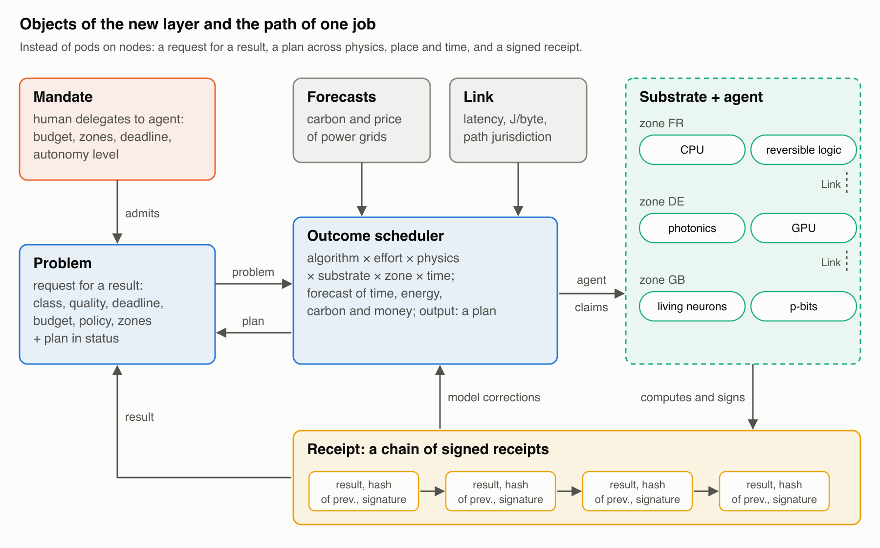
Objects of the new layer: a mandate admits a problem, the scheduler picks a method using grid forecasts and links, a substrate agent claims the work, and a signed receipt returns the result and model corrections
Lifecycle of work
- A human or an agent creates a
Problem. - The mandate is checked: the signature must belong to a registered human, and the validity period must include the current moment.
- The scheduler enumerates options by algorithm, effort, physics, substrate and start time. For each one it predicts time, energy, carbon and money, discards options that violate constraints, chooses according to policy and records the plan together with the trade-off frontier, that is, the set of options where you can gain on one axis only at the expense of another (the Pareto frontier). If the mandate requires approval, the plan waits for a human.
- The substrate agent sees a plan with its name on it, waits for the start time and claims the work with an optimistic write that checks the object’s version, so that of two agents competing for the same work only one succeeds.
- The agent computes, signs a receipt and writes the result. If the global level is unreachable, the receipt waits in a local on-disk queue.
- The receipt updates the quality distributions and the model corrections.
- If the agent goes silent before claiming the work, the work returns to the pool and is scheduled again.
Scheduling
A problem is described as an intent, and below it lives a multi-level representation modeled on MLIR, the compiler infrastructure in which a program is gradually lowered from general operations to instructions for specific hardware [86]: problem (optimization, inference, simulation) → algorithms (exact, annealing, sampling, approximate inference) → physics → concrete devices and data routes. The key point is that the model of computation is chosen by the scheduler, not by the programmer. The same optimization can be solved exactly on a CPU in an hour, approximately on an Ising machine in a second, or by sampling on p-bits, and each method has its own quality–energy–time curve. On a heterogeneous graph with floating prices this choice is an NP-hard problem, and nobody is going to solve it exactly. The workable path is heuristics generated and selected by AI and validated on a simulator or a digital twin. This is exactly how the ADRS approach works [60].
The decision space is algorithm × effort × physics × substrate × zone × start time. In the cost model, the number of operations (for annealing and the classifier it is known exactly before the run) is converted into time and energy using the substrate’s model, then multiplied by corrections learned from receipts and by the site’s power usage effectiveness factor (PUE; in the prototype this is a single constant of 1.2 for all sites). The energy of moving data over the link is added on top. Carbon is computed from the grid’s carbon intensity forecast for the execution window, and money from the price for that hour.
Quality is defined as the lower bound on the probability of reaching the target, based on observed runs (the Wilson interval). If there are no observations, the option is not offered. The constraints are the deadline, budget, zones, jurisdictions, mandate, calibration windows and capacity.
Scheduling is hierarchical, and all three levels work in the prototype. The global level, operating over minutes and hours, chooses the zone and start time based on grid forecasts and prices. The site level, operating in seconds, chooses the substrate and the moment within the zone, where it knows the queues. The local level lives in the substrate agent. If the device’s own recent results show that the planned effort no longer delivers the required quality with the required confidence, the agent raises the effort by one step, signs in the receipt what it actually ran, and the scheduler learns from that. The levels announce themselves through Lease objects, that is, leases that a level must renew regularly or else be considered gone. This is the same hierarchy used in power grid control, and the experiment on the testbed is described in Section 8.6.
The lower levels of this hierarchy must be able to live without the global level. A useful idea here comes from Dave Ackley of the University of New Mexico, who calls it robust-first computing [87]. His Movable Feast Machine model and the physical T2 Tiles describe a computer built from identical modules with no global clock and no master. Each tile talks only to its neighbors, computation emerges from a population of small “atoms” with local rules, structures continuously repair themselves, and correctness is achieved on a “best effort” basis. The machine can be grown indefinitely simply by adding tiles. Ackley rejects the von Neumann bargain, in which perfectly deterministic hardware lets software be fragile. In its pure form this is a philosophy rather than a ready-made architecture, because survivability is paid for with precision and debuggability. But for edge sites, robots and orbit, where the global level is unreachable by definition, local rules and neighbor coordination turn out to be the right form. Central guarantees remain where they cannot be done without, namely money, permissions and audit.
People often ask whether a quantum computer needs Kubernetes. Inside the quantum processor it does not, because that is one expensive machine with its own control stack. The unsolved problem lies around it, and researchers explicitly call scheduling of hybrid workloads a gap that has received less attention than software stack integration [88]. A quantum processor is a scarce, time-shared resource whose calibration drifts. Variational algorithms run a loop between a conventional processor and the quantum one (QPU) thousands of times, and their classical and quantum parts must be placed next to each other with minimal latency. Decoding for quantum error correction is an ordinary classical computation, but the answer is needed within microseconds, so it has to be computed next to the quantum processor. At PCSS (Poznań), for example, this is done with Slurm and CUDA-Q [20]. In our model the QPU becomes a substrate with calibration windows and a cryogenics cost, and the problem is stated as an outcome.
The agent as the first user
Principle P14 says that the API is designed first of all for a machine, while a human works with the same state through a console, reports and dashboards built on top of it. For a long time in the prototype this meant only that a problem could be described as an outcome rather than as a set of resources, and that one could ask for a plan without running anything. That is not enough. An agent differs from a human at the API not only in being a program. It calls the API thousands of times where a human would call it once. It retries requests, because a timeout tells it nothing about whether the work was accepted. And it does not read the response; it programmatically chooses its next step from it, so a response that only a human can understand is no response at all for an agent.
This led to three changes in the core. The first allows retries without double execution. The problem spec gained a requestID field. If the namespace already contains a problem with the same identifier, the scheduler does not schedule the copy; it rejects it and names the original in the status.duplicateOf field. An agent that did not wait for a response and resubmitted the problem under a different name gets a reference to the first attempt instead of a second bill for the same work. A dry run does not take up the identifier, because it runs nothing; neither does an attempt rejected as a duplicate or for exceeding the rate limit, since otherwise a retry after such a rejection would run into its own failure.
The second change provides rejections from which a program can decide what to do next. Previously the rejection reason was only text: “zone not allowed”, “budget exceeded”, “cannot meet the deadline”. The text remains, but next to it status.reasonCodes now holds stable codes: ZoneNotAllowed, JurisdictionNotAllowed, BudgetExceeded, QualityUnreachable, DeadlineTooShort, MandateInvalid, Duplicate, RateLimited and a few more. A code does not change when the wording changes. The scheduler records the code of every discarded option, not only of the twenty whose texts it keeps as samples. On receiving BudgetExceeded, an agent can raise the budget or relax the quality requirement; on DeadlineTooShort, it can move the deadline; on QualityUnreachable, it can understand that money is not the issue.
The third change protects the server from its own main user. The scheduler admits no more than a set number of new problems per namespace per minute, sixty by default; the excess is rejected with the code RateLimited and not scheduled. The apiserver protects itself from a flood of requests as such, but scheduling costs more than writing an object, because each problem requires enumerating algorithms, physics, locations and start time slots against grid forecasts. Work that returns to the pool after a substrate goes silent does not count as new.
In addition, an agent needs a way to discover all of this without knowing about CRDs and kubeconfig. For that there is now physis-mcp, a Model Context Protocol server through which the program hosting the agent discovers the available tools and calls them. There are five tools: list substrates together with their model parameters and provenance, get a plan with alternatives without running it, submit a problem (a requestID is required), check its state, and verify a substrate’s receipt chain against its published keys, current and revoked. Each tool has a strict schema, and an unknown field in the arguments is treated as an error rather than a constraint that can be silently dropped. The server has no privileges of its own. It calls the API under the agent’s credentials, and mandates, budgets and rate limits apply exactly as they do for any other client.
What remains open is the following. A receipt does not yet bind the result to a specific agent, because the requester’s name comes from an annotation that the client sets itself. A mandate is issued for a namespace, not for an agent, so two agents in the same namespace share a budget. The rate-limit window lives in the scheduler’s memory and is forgotten on restart. The system does not transfer money between agent and operator, although budgets in euros already exist and machine payment protocols have appeared. And the conformance suite does not yet test protection against repeated execution (idempotency), the codes or the rate limit; only unit tests cover them.
Network
- Addressing by identity, not by IP. Every problem, service and substrate has a cryptographic identity, that is, a key by which it can be unambiguously recognized and verified. Policy, audit and receipts speak in terms of identities, and IP becomes a transport detail on a single segment.
- A link is an object with a price. Latency, bandwidth, joules per byte, availability over time, jurisdiction of the path.
- Data movement is a scheduled operation. Data is content-addressed, and “move dataset X to zone Y” becomes a plan step with a price rather than a side effect of a launch.
- Transport by context. Inside a data center, RPC-oriented protocols such as Homa; between sites, QUIC; on intermittent links, store-and-forward. The application specifies delivery semantics, not a protocol.
- Policy by purpose and jurisdiction. The requirement “This data is processed only in EU zones by operators who have signed X” becomes a scheduling rule rather than a set of IP rules on nodes.
- Mutual authentication by default, because there is no longer a “trusted internal network”.
- No global flat address space. Connectivity between sites is described by links, not by the requirement that “everyone sees everyone”.
Here is what this looks like in objects. In the prototype a link is described by the Link resource, and the scheduler takes it into account in every decision where a problem has declared data:
apiVersion: physis.kuberoot.dev/v1alpha1
kind: Link
metadata: {name: de-fr}
spec:
  from: DE
  to: FR
  jPerByte: 4.77e-06          # energy to transfer one byte
  latencySeconds: 0.01
  bytesPerSecond: 1.25e+09    # 10 Gbit/s
  pathJurisdictions: [EU]     # jurisdictions the path crosses
  source: "ref:aslan2018 …; bandwidth and latency: assumption"
A problem declares where its data lives, how much of it there is, and under which jurisdictions it may be processed:
spec:
  dataZone: GB
  dataBytes: 1.0e+9
  jurisdictions: [EU]
From there three rules apply, and all three are covered by tests:
- a transfer costs exactly as much energy as the link says, and is counted toward carbon at the average carbon intensity of the path’s endpoints;
- work will not start before the data can arrive: transfer time equals
dataBytes / bytesPerSecondplus latency; - if there is no link between the zones, or the path crosses a jurisdiction the problem has not allowed, the option is unavailable even if the substrate at the other end is allowed. Data from the UK with an “EU only” requirement will not go to France, because the path crosses the UK jurisdiction.
What from today’s stack works as a foundation, and what is replaced:
| Today | Role in the new layer |
|---|---|
| eBPF-based network traffic processing (for example, Cilium) | Stays as fast local transport and the means of enforcing policy at a site |
| Gateway API | Stays as the standard way to describe ingress traffic from outside; routing inside the substrate marketplace is by identities and links |
| SPIFFE (a standard for cryptographic service identities) and similar schemes | The foundation for identity-based addressing and mutual authentication |
| Multi-Cluster Services | Replaced by links as objects and data movement as a plan step |
| kube-proxy and service virtual IPs | Become a detail of a single site rather than the model for the whole system |
| NetworkPolicy by IP and labels | Replaced by policy by identity, purpose and jurisdiction, enforced by the scheduler |
The migration path is as follows. First, links and the cost of transfer appear as objects alongside the existing network, and the prototype already does this. Next, data movement becomes a plan step with content addressing. Then identity replaces IP in policies and receipts. Meanwhile the cluster’s flat network can stay inside a single site for as long as needed.
Identity-based addressing: what already works
Until now, of the seven points in the network section the prototype implemented the link as an object with a price and the jurisdiction of the path, while identity-based addressing and mutual authentication remained a description. Their core now works for substrates and can be verified with tests and on the testbed.
A substrate’s identity is the key the agent already had. The agent signs receipts with an Ed25519 key, publishes it in status.publicKey and keeps it across restarts. The same key now also serves as a network address. No new credentials need to be issued, and data is carried by the same identity that signs the result. The address is written as physis: followed by the base32 encoding of the full key plus two checksum bytes, for example physis:mvmz7oylrc5wkjhfmz2jlai2kn3tuxjp37nxegq2tpv42btcy2ek7zq. The address contains the whole key, not a prefix of it. This makes the address self-certifying. To confirm that the peer is the one named, you don’t need to look anything up or trust anyone — not DNS, not an IP address, not the API server. A typo in the address produces a checksum error, not someone else’s key.
The agent itself reports where the substrate can currently be reached. If it is started with the -listen flag, a list of endpoints appears in the substrate’s status:
status:
  publicKey: 65599fbb...
  endpoints:
  - {transport: https, address: 10.0.3.7:7443}
The resolver, that is, the identity lookup service, finds the substrate, its zone, jurisdiction and endpoints. A key retired during rotation leads nowhere and is only good for verifying old receipts. If the same key is claimed by two substrates, the resolver refuses to choose, because the jurisdiction of such an identity is ambiguous, and a public key copied into someone else’s object must not redirect anything. Endpoints here serve only as hints and are not trusted. The key is verified on every connection, and a stale or forged address leads to a refusal, not to someone else’s data.
Mutual authentication rests on TLS 1.3 on both sides, where the certificate key is the identity key. The certificates are self-signed, and neither the certificate authority, nor the name, nor the validity period is checked — only the key. TLS 1.3 is itself a challenge–response scheme, because each side signs the handshake transcript, which includes the peer’s random nonce, with its certificate’s private key. The caller verifies that the key in the certificate belongs to the party it meant to reach; the receiving side learns from the certificate who has connected. We chose this path rather than signing each response over plain HTTP because TLS provides encryption, replay protection and per-byte integrity through the standard library, leaving only the key match to check.
Data transfer between agents is built on top of this. Agent A requests an object by name from identity B. The client finds B through the resolver, connects, verifies the key and fetches the object in chunks. The first chunk arrives together with the content hash, the remaining ones are requested on the condition that the hash has not changed, and at the end the whole object is checked against the hash. If B has moved, restarted at a different address, or its old address has been taken by another machine, the connection either drops or fails the key check. A then finds B again by identity and resumes from the last byte received. A refusal from B itself, for example on policy grounds, is final, and retrying is pointless. The test runs exactly this scenario. B moves in the middle of the transfer, and a third identity takes over its old port, serving different bytes under the same name; A detects the substitution by the key, finds B again and receives B’s bytes.
The decision “may this be sent” is made by the sender, and it is made based on the recipient’s identity, not its address. The rule is the same one the scheduler applies to data paths. The jurisdiction of the recipient’s operator must be among those allowed for this data, and if links are declared in the cluster, there must be a link between the sender’s and recipient’s zones whose path does not cross forbidden jurisdictions. An identity with no substrate behind it receives nothing. If the links cannot be read, the transfer is denied, because an unknown network is not considered open. The scheduler and the agent now share the code for this rule, so they cannot diverge.
For a substrate behind NAT that cannot be dialed but can itself reach the API server, there is a fallback through a mailbox of small signed messages. A posts a request with its signature and a fresh nonce; B picks it up, verifies A’s signature, applies the same policy and posts a response with its own signature that repeats A’s nonce. A response cannot be forged on behalf of B, a request cannot be forged on behalf of A, and an old response cannot be replayed. The response is limited to 256 KiB. The protocol is written and tested against an in-memory mailbox, but the mailbox on API objects is not built yet, and the agent does not advertise this connection method.
On the node-free testbed it looks like this. Substrate B in zone DE under EU jurisdiction serves a 3 MB file that is allowed for the EU only. Agent A from FR receives it, and the bytes match. Agent C from the UK gets a refusal: “substrate c is under UK jurisdiction, data allowed for [EU]”. B restarts on a different port, publishes a new endpoint, and A again receives the file at the same physis:… address. On a four-node kuberoot cluster the experiment was repeated across machines: substrate B on one node served 3 MB to agent A on another node, the hash matched, and agent C with UK jurisdiction on a third node was refused (results/identity-cluster.txt). All of this is off by default. Without -listen the agent opens no port and publishes nothing, so existing testbeds and the conformance suite are unaffected.
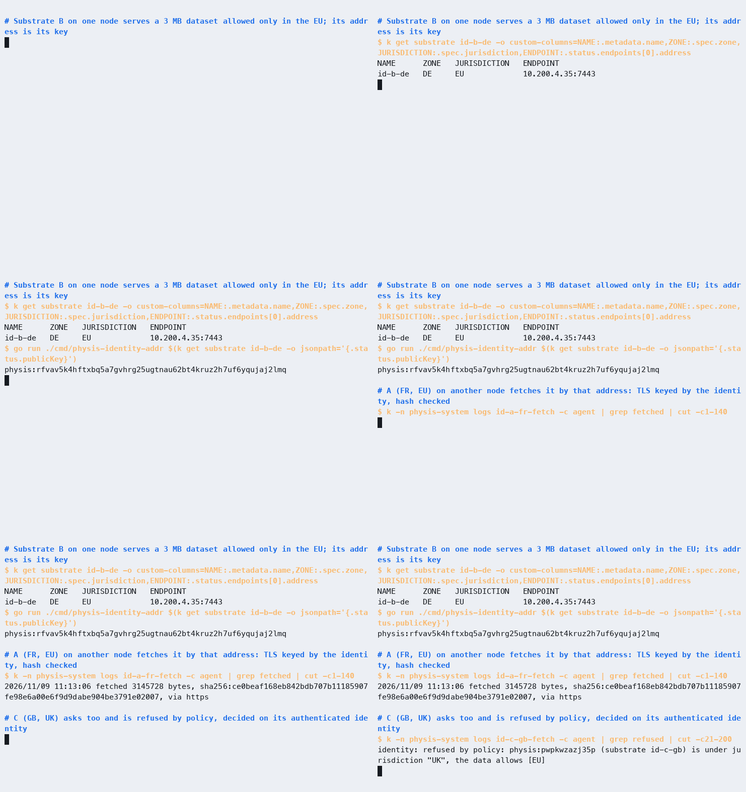
Identity-based networking on a kuberoot cluster: a substrate address derived from its key, data retrieval on another node, and a refusal on jurisdiction grounds
What this proves and what it does not. A peer that has completed the handshake holds the identity’s private key. An API server, DNS or router that lies about endpoints can disrupt a transfer, but cannot make A accept bytes that did not come from B, or make B hand data to the wrong identity. The substrate’s jurisdiction, however, comes from what is declared about it in the API, because authentication proves who the recipient is, not where it is. Messages through the mailbox are signed but not encrypted. The whole object is held in memory, and storage is a directory of files. This is a protocol prototype, not a production-ready data transfer mechanism.
Still in the design stage is the mailbox on API objects with encryption for the recipient. So is transfer as a plan step. The scheduler already computes the cost and time of a transfer but does not yet order it, and data is still addressed by name rather than by content end to end. Not yet implemented are identities for workloads, datasets and mandates, not just substrates, and a SPIFFE-compatible form for existing service meshes, which take care of encryption and routing between services. Transport is not yet chosen by context. There is only one, HTTP/1.1 over TLS 1.3 over TCP, while QUIC between sites, Homa inside the data center and multipath transfer exist only in the design. Store-and-forward over the Bundle Protocol for links that are down for hours is not implemented either, because chunked resumption survives a break of seconds or minutes, but not hours. kube-proxy and CNI have not been replaced. The identity channel runs on top of whatever IP network the site has, and the pod network, services and NetworkPolicy are untouched. And there is no proof of location, so jurisdiction is declared rather than attested.
The migration path described above has advanced by one step: identity has already replaced the IP address where substrates transfer data to each other and decide whether it may be sent.
The cloud as a substrate marketplace, and sovereignty
If the physics varies and belongs to different owners in different countries, “cloud” no longer means a provider with identical servers. The cloud becomes a marketplace of substrates connected through one common interface. Providers (one with an Ising machine in Poland, another with a quantum processor in Germany, another with analog accelerators in France) publish a Substrate with a model, a price and a jurisdiction. The scheduler chooses by outcome and cost. Sovereignty (the operator’s jurisdiction, data location, data path, substrate attestation) becomes a hard scheduling constraint rather than a checkbox in a contract. Hybrid then stops being an architecture of “a bit of our own, a bit of public” and becomes the norm, because any problem can go to any physics at any owner, as long as the mandate allows it and it pays off.
Compatibility
The new entities are implemented as CRDs on top of a standard apiserver, so kubectl, RBAC and GitOps (managing a cluster through descriptions stored in Git) work with them out of the box. Pods and containers remain the “Linux processes” substrate for legacy software, but stop being the center of the system.
The bridge from today’s device description is in place. A DRA driver publishes devices in a ResourceSlice; physis-dra-bridge turns each recognized device into a Substrate. DRA has no cost model, so a driver can add one as attributes in the physis.kuberoot.dev domain; whatever it specifies is cited as a reference to the driver, and everything it does not specify is taken from the reference model for that physics and marked as an assumption. The bridge writes only the description, and the substrate comes alive when an agent serves it (physis-agent -adopt), so a device that is described but not served by anyone never ends up in a plan. To make this work, the scheduler now builds each substrate’s model from what the substrate publishes about itself rather than from a built-in table.
And a substrate agent no longer has to be a container, or even a Linux process. The device core — computation and signing with a key that lives only there — has been moved into a separate program, physis-device, which exchanges JSON messages, one per line, over standard input and output and requires no network, no sockets and no Linux. It compiles to WebAssembly (WASI) and runs in a sandbox; the agent around it handles only the networking and never sees the key. The same protocol works for a microcontroller on a serial port. For kuberoot there is a container-free distribution (deploy/kuberoot-distro), in which a node runs only the kernel, init, the API server with its own storage, the controller manager, the node API and physis itself as node services, without kubelet, containerd or pods. It is built, booted on a server and passes conformance (Section 8.6).
7. The physis prototype
To test the design, we built a prototype. We called it physis, the Greek word for “nature” in the sense of “the way a thing is made.” It is roughly eleven thousand lines of Go under the Apache 2.0 license. The prototype implements exactly the objects described above on top of a stock kube-apiserver and installs into kuberoot as a kubepkg package or a Helm chart; the scheduler and the agents run as ordinary pods.
What is inside
| Component | What it does |
|---|---|
physis-scheduler | Watches Problem objects, checks mandates, plans across live substrates and fresh grid forecasts, and records the plan along with its alternatives. It executes nothing itself and binds nothing to nodes |
physis-agent | One agent per substrate. Publishes the substrate’s model, sends a regular liveness signal (heartbeat), claims the work planned for that substrate, executes it, signs a receipt and reports the result. An ordinary Deployment with no node affinity |
physis-conformance | A suite of 17 black-box tests (section 9) |
physis-calibrate | Runs every algorithm on every physics and builds quality distributions |
physis-sim | A digital twin: the same scheduler logic run over a stream of problems and a quarter of real grid data |
physis-data | Loads grid data |
CRDs Substrate, Problem, Receipt, Mandate, Link | The layer’s objects on top of a stock kube-apiserver; Link describes the network between zones as paths with a cost |
The key architectural decision is that the code contains not a single reference to Node objects. The RBAC roles granted to physis give no access to nodes or to pods, and conformance test TC-02 verifies this. Work is claimed through an optimistic write to the problem’s status: of two agents competing for the same work, the one whose write arrives with the current object version wins.
Two problems
A fair comparison of physics requires problems that map onto them naturally.
MaxCut asks for a partition of a graph’s vertices into two groups that maximizes the total weight of the edges between the groups. It is a classic NP-hard problem and, at the same time, the canonical problem for Ising machines. If each vertex is assigned a “spin” of ±1, the cut equals the energy of an Ising model up to sign and a constant. We use the standard Gset collection (Helmberg and Rendl), specifically graphs G1, G2, G11, G14, G22 and G43, which range from 800 to 2000 vertices. For G1, G2 and G22 we confirmed the published best-known cuts in two independent sources [89]. We also use small random graphs with 12–20 vertices, for which the exact optimum can be found by exhaustive search.
The main way the prototype solves MaxCut is simulated annealing. The algorithm flips spins one at a time, almost always accepting changes that improve the cut and accepting changes that worsen it less and less often as a notional “temperature” falls. The temperature is lowered gradually, the way metal cools slowly, which is where the name comes from: early on the search wanders freely across solutions, and toward the end it settles into a good one. The number of steps sets the effort: more steps yield a better cut and a more expensive computation. The same dynamics run on the digital Ising machine and on superconducting and reversible logic, while p-bits and the optical Ising machine search for the energy minimum in a similar but physically distinct way.
Classification of handwritten digits from the UCI dataset (1,797 test images of 8×8 pixels) [90] with a linear model. It reduces to matrix-vector multiplications, the native operation of analog in-memory computing, photonics and neuromorphic chips.
Eighteen physics
Only two of the prototype’s physics are real: the CPU and the GPU. Twelve physics are described below. Six more were added later and are covered in section 8.6: a systolic tensor array (FP8, MXFP4, int8), processing in DRAM, a dataflow processor, stochastic and hyperdimensional computing, and a coarse-grained reconfigurable array (CGRA). The GPU role is played by the Apple M4 graphics processor in a laptop. The classifier runs on it through MLX, Apple’s machine learning library, and device time is measured (see section 8.6 for details). The remaining sixteen physics are emulated. The algorithm that a given physics would execute is genuinely run on the CPU and counts its elementary operations, and a device model converts the operation count into the time and energy of the real machine. Every model parameter carries its provenance: a measurement, a published figure with a citation, or an explicit assumption with a range that is later tested by sensitivity analysis.
This is a deliberate choice, so it is worth stating plainly what it shows. Emulation does not prove that, say, p-bits are 100 times more efficient than a CPU. It tests the mechanism: whether the layer can describe different physics, choose among them by result and cost, learn from receipts and respect constraints. Once a real machine is connected, its model is recalibrated from receipts (see section 8.4).
Each physics runs its own algorithms:
- CPU: exact enumeration (up to 24 vertices), local search with restarts, Metropolis annealing; a double-precision classifier.
- Digital annealing, superconducting (SFQ) logic and reversible (adiabatic) logic run the same Metropolis annealing, that is, identical dynamics on different physics, and therefore produce identical quality.
- p-bits: Gibbs sampling with increasing inverse temperature, because that is how probabilistic computers operate.
- Coherent optical Ising machine: amplitude dynamics of parametric oscillators with saturation, noise and feedback.
- Quantum processor: QAOA (the quantum approximate optimization algorithm) with a linear angle schedule on a full state-vector emulator, up to 20 qubits; two-qubit gate errors are modeled with a global depolarizing model (0.5% per gate).
- Analog memory and photonics: a classifier with weight quantization, programming error, read noise and an ADC.
- Neuromorphic chip: spike-based classification with rate coding, where a number is carried by the pulse frequency; more time steps mean higher accuracy and higher cost.
- Living neuron culture: reservoir computing. A noisy random recurrent network (an echo state network) stands in for the culture, and a linear readout is trained on a conventional computer. This is how cultures are used today, because a culture’s synapses cannot be trained by gradient descent.
Device models (the table is generated from the prototype’s code):
| Physics | Emulated | Operations/s | Energy per operation, J | Power, W | Load, s | Load, J | Calibration | Capacity |
|---|---|---|---|---|---|---|---|---|
| cpu | no | 5e+07 (1e+07–2e+08) · measured | — | 6.04 (3–9) · ref:amd-9454p | — | — | — | 1073741824 |
| ising-digital | yes | 4e+09 (1e+08–4e+10) · assumption | — | 40 (15–150) · assumption | 0.002 (0.0005–0.02) · assumption | 0.08 (0.01–1) · assumption | — | 100000 |
| pbit | yes | 1e+11 (1e+09–1e+12) · assumption | 2e-15 (1e-15–2e-14) · ref:singh2024 | — | 0.001 (0.0001–0.01) · assumption | 0.01 (0.001–0.1) · assumption | — | 20000 |
| analog-imc | yes | 3.16e+13 (1e+12–3.16e+13) · ref:legallo2023 | 2.05e-13 (2e-14–2e-12) · ref:legallo2023 | — | 0.05 (0.01–1) · assumption | 0.001 (0.0001–0.01) · assumption | 30 s every 1 h | 4194304 |
| qpu | yes | 5e+03 (1e+03–2e+04) · assumption | — | 2.6e+04 (1.5e+04–3e+04) · ref:arute2019supp | 2 (0.5–30) · assumption | 5.2e+04 (7.5e+03–9e+05) · assumption | 900 s every 6 h | 20 |
| optical-ising | yes | 1e+09 (1e+08–1e+10) · assumption | — | 1e+03 (200–3e+03) · assumption | 0.01 (0.001–0.1) · assumption | — | — | 100000 |
| sfq | yes | 2e+10 (1e+09–1e+11) · assumption | 7.4e-12 (7.4e-13–7.5e-10) · assumption | 740 (74–3.75e+04) · assumption | 0.001 (0.0001–0.01) · assumption | — | — | 50000 |
| adiabatic | yes | 2e+09 (5e+07–2e+10) · assumption | 7e-09 (1e-09–9e-09) · assumption | — | 0.002 (0.0005–0.02) · assumption | — | — | 100000 |
| neuromorphic | yes | 1e+10 (1e+09–1e+11) · assumption | 2.36e-11 (4e-12–2.5e-11) · ref:loihi | 1 (0.1–5) · assumption | 0.01 (0.001–0.1) · assumption | — | — | 1048576 |
| photonic | yes | 1e+12 (1e+11–1e+13) · assumption | 2.7e-13 (2e-14–2e-12) · ref:photonic2024 | 5 (1–20) · assumption | 0.001 (0.0001–0.01) · assumption | — | — | 65536 |
| organoid | yes | 3e+04 (3e+03–3e+05) · assumption | — | 30 (20–100) · ref:cl1power | 1 (0.1–10) · assumption | — | 3600 s every 24 h | 1048576 |
| systolic | yes | 4.6e+13 (4.6e+12–4.6e+13) · ref:jouppi2017tpu | — | 40 (30–75) · ref:jouppi2017tpu | 0.001 (0.0001–0.01) · assumption | 0.04 (0.003–0.75) · assumption | — | 1073741824 |
| pim-dram | yes | 6e+11 (6e+10–6e+11) · ref:kwon2021fimdram | 4.6e-11 (2e-11–9.3e-11) · assumption | — | 0.0001 (1e-05–0.001) · assumption | — | — | 1073741824 |
| dataflow | yes | 3.75e+14 (3.75e+13–3.75e+14) · ref:abts2020tsp | — | 300 (150–400) · assumption | 0.0001 (1e-05–0.001) · assumption | 0.03 (0.0015–0.4) · assumption | — | 1073741824 |
| stochastic | yes | 1e+12 (1e+11–1e+13) · assumption | 5e-15 (1e-15–3e-14) · assumption | — | 0.0001 (1e-05–0.001) · assumption | — | — | 1073741824 |
| hdc | yes | 1e+12 (1e+11–1e+13) · assumption | 6e-16 (2e-16–5e-15) · assumption | — | 0.0001 (1e-05–0.001) · assumption | — | — | 1073741824 |
| cgra | yes | 6.15e+12 (1.1e+12–6.15e+12) · ref:podobas2020cgra | — | 49 (20–49) · ref:podobas2020cgra | 0.0001 (1e-05–0.01) · assumption | 0.0049 (0.0002–0.49) · assumption | — | 1073741824 |
| gpu | no | 5e+09 (8e+08–7e+09) · measured | — | 8 (3–20) · assumption | 0.004 (0.003–0.05) · measured | 0.032 (0.009–1) · assumption | — | 1073741824 |
A few notes on the table. The quantum processor’s energy is computed as the power of the installation including cryogenics (about 26 kW [21]) multiplied by time, not as energy “per operation,” and it includes two seconds of problem loading, 52 kJ, which dominates the total on small problems. Likewise, for p-bits (10 mJ) and digital annealing (80 mJ), most of the energy on small problems goes into loading rather than computation. For reversible logic we take only the 30 percent saving from Vaire’s work [15]; the baseline energy of a conventional annealer it is measured against is our own assumption. For superconducting logic, switching energy is scaled up to wall-plug energy with a cooling factor of 740 W per watt of heat at 4 K, since that is what installations based on Collins and Brayton cycles typically require [18]. The Carnot limit is about 74 W/W, the best installations come in under 400 W/W [17], and small cryocoolers require 5–7.5 kW/W [18]. For the living culture, the main cost is the life-support system rather than the neurons themselves, and we use 30 W, with headroom over the 20 W quoted for the device [22]. This is exactly what makes them interesting for the scheduler: each physics has its own cost profile.
Calibration: what actually comes out
Before planning, every “algorithm × effort × physics” combination is run on all instances with 12 different random number generator seeds (exact solvers once). This produced 6,405 calibration records in total, because a single annealing emulation counts for every physics with the same dynamics. CPU time is measured, core power is taken from the EPYC 9454P specification [91], and everything else is computed by the model. Here is part of the results, sorted by energy:
MaxCut G22 (2000 vertices, 19,990 edges), quality as a fraction of the best-known cut of 13,359
| Physics | Algorithm / effort | Quality (mean ± std. dev.) | Device time | Device energy |
|---|---|---|---|---|
| adiabatic | anneal / w300 | 0.9951 ± 0.0015 | 2.3 ms | 4.2 mJ |
| pbit | pbit / w300 | 0.9922 ± 0.0015 | 1.01 ms | 10 mJ |
| pbit | pbit / w3000 | 0.9969 ± 0.0013 | 1.06 ms | 10 mJ |
| pbit | pbit / w30000 | 0.9995 ± 0.0011 | 1.6 ms | 10.3 mJ |
| sfq | anneal / w300 | 0.9951 ± 0.0015 | 1.03 ms | 22.2 mJ |
| adiabatic | anneal / w3000 | 0.9987 ± 0.0013 | 5 ms | 42 mJ |
| cpu | local / s10 | 0.9605 ± 0.0022 | 10.7 ms | 64.3 mJ |
| ising-digital | anneal / w300 | 0.9951 ± 0.0015 | 2.15 ms | 86 mJ |
| ising-digital | anneal / w3000 | 0.9987 ± 0.0013 | 3.5 ms | 140 mJ |
| cpu | anneal / w300 | 0.9951 ± 0.0015 | 25.8 ms | 156 mJ |
| sfq | anneal / w3000 | 0.9987 ± 0.0013 | 1.3 ms | 222 mJ |
| optical-ising | cim / r200 | 0.9286 ± 0.0035 | 10.4 ms | 400 mJ |
| adiabatic | anneal / w30000 | 0.9999 ± 0.0001 | 32 ms | 420 mJ |
| cpu | local / s100 | 0.9639 ± 0.0017 | 105 ms | 634 mJ |
| ising-digital | anneal / w30000 | 0.9999 ± 0.0001 | 17 ms | 680 mJ |
| cpu | anneal / w3000 | 0.9987 ± 0.0013 | 261 ms | 1.58 J |
| optical-ising | cim / r1000 | 0.9649 ± 0.0033 | 12 ms | 2 J |
| sfq | anneal / w30000 | 0.9999 ± 0.0001 | 4 ms | 2.22 J |
| optical-ising | cim / r5000 | 0.9833 ± 0.0021 | 20 ms | 10 J |
| cpu | anneal / w30000 | 0.9999 ± 0.0001 | 2.46 s | 14.9 J |
MaxCut on random 20-vertex graphs, quality as a fraction of the exact optimum
| Physics | Algorithm / effort | Quality (mean ± std. dev.) | Device time | Device energy |
|---|---|---|---|---|
| adiabatic | anneal / w300 | 1.0000 ± 0.0000 | 2 ms | 42 µJ |
| cpu | local / s10 | 0.9978 ± 0.0079 | 16.5 µs | 99.6 µJ |
| sfq | anneal / w300 | 1.0000 ± 0.0000 | 1 ms | 222 µJ |
| adiabatic | anneal / w3000 | 1.0000 ± 0.0000 | 2.03 ms | 420 µJ |
| cpu | anneal / w300 | 1.0000 ± 0.0000 | 110 µs | 663 µJ |
| cpu | local / s100 | 1.0000 ± 0.0000 | 129 µs | 782 µJ |
| sfq | anneal / w3000 | 1.0000 ± 0.0000 | 1 ms | 2.22 mJ |
| optical-ising | cim / r200 | 0.9619 ± 0.0342 | 10 ms | 4 mJ |
| adiabatic | anneal / w30000 | 1.0000 ± 0.0000 | 2.3 ms | 4.2 mJ |
| cpu | anneal / w3000 | 1.0000 ± 0.0000 | 1.01 ms | 6.09 mJ |
| pbit | pbit / w300 | 1.0000 ± 0.0000 | 1 ms | 10 mJ |
| pbit | pbit / w3000 | 1.0000 ± 0.0000 | 1 ms | 10 mJ |
| pbit | pbit / w30000 | 1.0000 ± 0.0000 | 1.01 ms | 10 mJ |
| optical-ising | cim / r1000 | 0.9894 ± 0.0131 | 10 ms | 20 mJ |
| sfq | anneal / w30000 | 1.0000 ± 0.0000 | 1.03 ms | 22.2 mJ |
| cpu | exact / full | 1.0000 ± 0.0000 | 8.4 ms | 50.7 mJ |
| cpu | anneal / w30000 | 1.0000 ± 0.0000 | 9.97 ms | 60.2 mJ |
| ising-digital | anneal / w300 | 1.0000 ± 0.0000 | 2 ms | 80.1 mJ |
| ising-digital | anneal / w3000 | 1.0000 ± 0.0000 | 2.01 ms | 80.6 mJ |
| ising-digital | anneal / w30000 | 1.0000 ± 0.0000 | 2.15 ms | 86 mJ |
| optical-ising | cim / r5000 | 0.9964 ± 0.0071 | 10.1 ms | 100 mJ |
| qpu | qaoa / p4s256 | 0.9564 ± 0.0309 | 2.05 s | 5.33e+04 J |
| qpu | qaoa / p8s1024 | 0.9555 ± 0.0312 | 2.2 s | 5.73e+04 J |
Classification of 1,797 UCI handwritten digits, quality as accuracy relative to the exact classifier
| Physics | Algorithm / effort | Quality (mean ± std. dev.) | Device time | Device energy |
|---|---|---|---|---|
| photonic | analog / w4 | 0.9958 ± 0.0035 | 1 ms | 6.06 µJ |
| neuromorphic | spiking / t8 | 0.9898 ± 0.0022 | 10.3 ms | 347 µJ |
| analog-imc | analog / w4 | 0.9771 ± 0.0051 | 50 ms | 1 mJ |
| neuromorphic | spiking / t32 | 0.9983 ± 0.0015 | 11.1 ms | 1.39 mJ |
| cpu | exact-fp / fp64 | 1.0000 ± 0.0000 | 726 µs | 4.39 mJ |
| neuromorphic | spiking / t128 | 1.0002 ± 0.0012 | 14.5 ms | 5.55 mJ |
| organoid | reservoir / s8 | 1.0365 ± 0.0028 | 145 s | 4.31e+03 J |
| organoid | reservoir / s20 | 1.0340 ± 0.0019 | 360 s | 1.08e+04 J |
The calibration already reveals things the scheduler later exploits:
- On large graphs, the same annealing on specialized machines costs 2–40 times less than on the CPU at equal quality, and p-bits with their own sampling algorithm cost up to three orders of magnitude less.
- On small graphs, the cheapest CPU option beats almost all specialized machines, because for many of them the fixed cost of loading the problem exceeds the computation itself. The exception is reversible logic, whose model has no loading energy.
- On 20-vertex graphs the quantum processor reaches 95.6% of the optimum on average (gate errors eat part of the quality) and spends about 53 kJ, because the cryogenics run for the entire duration of the problem. Exact enumeration on the CPU finds the optimum for 51 mJ, roughly a million times cheaper. This model does not say that quantum computers are useless. It says that for MaxCut on 20 vertices they make no sense, and the scheduler has to see that.
- The living culture classifies digits even more accurately than the linear model, because the reservoir is a nonlinear feature expansion. But for 1,797 images it needs about six minutes and about 10 kJ of life-support energy, roughly a million times more than any other physics on this problem.
The scheduler
For each problem, the scheduler enumerates algorithm × effort × substrate × start time. Deferrable work is considered in 15-minute steps all the way up to the deadline. For each option, it:
- counts operations, exactly and before execution for annealing, QAOA and classification;
- converts them into time and energy using the substrate’s model, multiplies by corrections learned from receipts and by the PUE (a single constant of 1.2 in the prototype);
- adds the energy of data transfer if the substrate is outside the data’s zone;
- checks calibration windows and intervals already reserved on the substrate;
- takes the Wilson lower bound on the probability of reaching the required quality from observed runs (an option with no observations is not proposed);
- computes carbon from the forecast grid carbon intensity for the execution window, and money from the hourly day-ahead market price;
- discards everything that violates the deadline, budget, zones, jurisdictions or mandate.
It then picks the minimum according to the policy (minimum carbon, energy, money or time) and keeps the Pareto frontier, the set of options none of which is worse than another on every axis at once.
Grid data
We compute carbon intensity for Germany, France and Poland ourselves from the generation mix published by Energy-Charts (Fraunhofer ISE) [92], using the IPCC AR5 median life-cycle emission factors [93]. For these countries our forecast is naive: we take the same quarter-hour from the previous day. For Great Britain we use the grid operator’s official forecast and actuals [94]. Prices come from the day-ahead market (CC BY 4.0, Bundesnetzagentur | SMARD.de); there is no open price for Great Britain. We excluded Spain because its price data may not be used beyond private purposes.
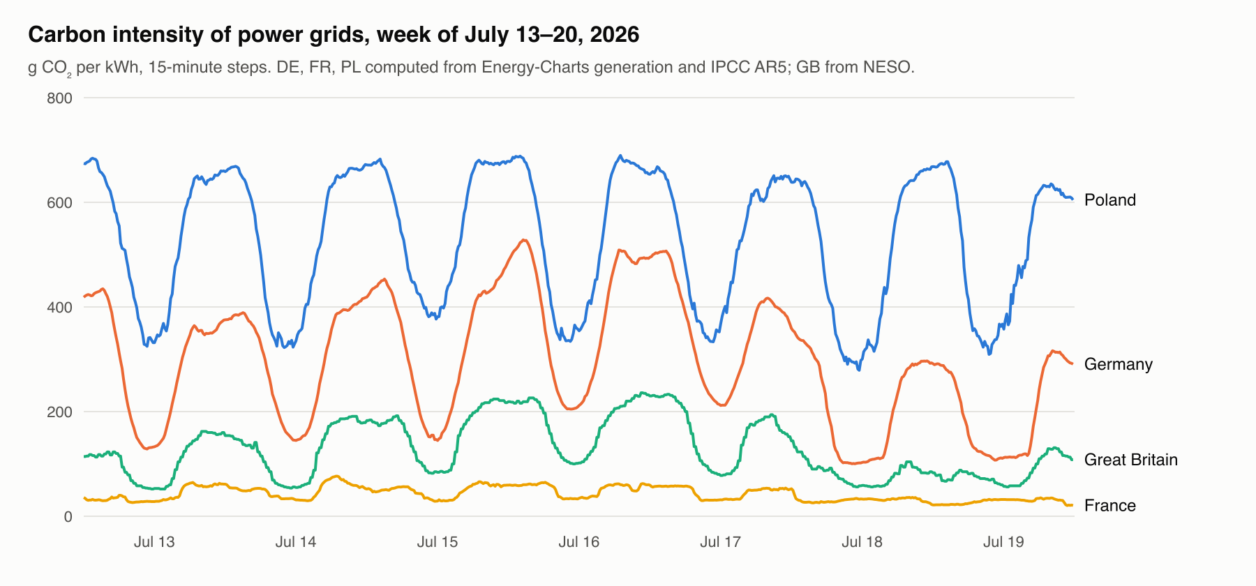
Carbon intensity of four power grids over one week
The averages for the third quarter of 2026 show how different these grids are. The daily rhythm is clearly visible in the chart. During the day, when the sun is shining, intensity in Germany drops by a factor of two and a half and in Poland by almost half, then rises again in the evening; this is where the benefit of shifting flexible work in time comes from. Nuclear-heavy France sits at about 39 g CO₂ per kWh, Great Britain at about 118, Germany at about 293, and coal-heavy Poland at about 505. The mean error of our naive forecast for Germany is 67 g/kWh, while the official British forecast’s error is 12. Below we show what this difference costs.
Receipts and mandates
On first start, each agent generates an Ed25519 key and publishes the public half in its substrate’s status. A receipt records: who made the request and under which mandate; the instance hash, algorithm, effort, agent build and random number generator seed; the substrate, the physics and whether it is emulated; the hash and quality of the result; the operation count, device time and energy, host CPU time, grid intensity and emissions. The receipt is signed and contains the hash of the same agent’s previous receipt. A receipt cannot be altered or deleted unnoticed, because either the signature or the next link in the chain breaks. The Receipt object itself is immutable at the API level, enforced by a CRD validation rule.
A mandate is signed by a human. It delegates a namespace, a daily budget in joules, euros and grams of CO₂, zones, a validity period and an autonomy level: “manual” requires approval of every plan; “augmented” requires approval of plans above a threshold; “directed” lets agents act on their own within the budget. Human keys are registered in the system’s control plane, and the signature is checked for every problem.
8. How we tested it
8.1. Methodology
We tested at three levels, and each one plays its own role.
Calibration on a real processor. Every “algorithm × effort × physics” combination was run on all instances with 12 random number generator seeds, which produced 6405 calibration records in total. These are real computations: cuts are actually computed, classifiers actually classify, and quality is measured against best-known results and exact solutions. CPU time is measured; time and energy for the other physics are computed by a model from the operation count. Twelve repetitions were not an arbitrary choice. With five repetitions, the scheduler refused to schedule G22, because five successes out of five give a Wilson lower bound of 0.83, while 0.9 was required. The system declined to promise what it had not verified well enough, exactly as principle P5 demands.
A digital twin on real power grid data. The simulator runs the same scheduler code. A stream of roughly 13 thousand problems per quarter arrives twice as often during the day as at night. Half of the problems are interactive (a 60-second deadline, no waiting allowed) and half are batch (a deadline of 2 to 24 hours, waiting allowed). Every fifth problem may run only in the EU, and every tenth only in the zone where its data lives. We used two quarters of 2026, the first (winter) and the third (summer), with data for Germany, France, Poland and the United Kingdom at 15-minute resolution. The substrate fleet consists of 16-slot CPU pools in each country plus one machine of each of the ten special physics, held by different “owners” in different countries. The scheduler sees only the forecast, while carbon and money are charged according to the actual hours in which the work really ran. The execution outcome comes from calibration: quality is sampled at random from the values actually observed for that combination, and costs come from the model with a ±10% spread (log-normal noise). Each policy is run five times with different generator seeds; we report the mean and the 5–95% range.
Live testbeds. The first testbed is a real kube-apiserver 1.37 with etcd and not a single node, with the scheduler and 14 agents running as processes. Its purpose is to show that the system has no need for Node objects at all. The second testbed is the kuberoot
edgecluster. The distribution was built from source for arm64 (Linux kernel 6.18.55, DRBD modules, root file system, 403 MB image) and booted in QEMU with hardware virtualization. The machine comes up as a single-node cluster on Kubernetes 1.37.1, and physis is installed into it from a Helm chart shipped in a kubepkg package (manifests are generated from the chart and applied with kubectl). The physis image is placed in a registry on the node itself, and containerd pulls it from the node’s own local address. All 15 physis components (the scheduler and 14 agents) run on kuberoot as pods. Both testbeds used fresh power grid forecasts for the day of the run, a stream of 120 problems in real time, and the conformance suite. Two more testbeds, multi-node kuberoot clusters on which we tested a real network partition, are described in section 8.6.
We compared seven policies:
| Policy | What it is |
|---|---|
| Kubernetes today | CPU only, only in the data’s zone, immediately, as fast as possible. This is how most clusters work |
| Carbon-aware, CPU only | CPU only, but in any permitted zone and shifted in time toward minimum carbon — this is how today’s “green” schedulers work |
| Mixed physics, speed only | All physics, but the goal is to finish as early as possible, with no regard for energy |
| physis: minimum energy | All physics, all zones, no waiting |
| physis: minimum carbon | All physics, all zones, waiting allowed up to the deadline |
| physis: minimum money | The same, with money as the goal |
| Oracle | Like “minimum carbon,” but sees the actual intensity instead of the forecast: an upper bound on what a perfect forecast can deliver |
8.2. The main result
The third quarter of 2026, about 13 thousand problems per run, five runs:
| Policy | Energy, Wh | Carbon, g CO₂ (5–95%) | Versus “Kubernetes today” | Mean wait | Missed deadlines | Quality shortfall |
|---|---|---|---|---|---|---|
| Kubernetes today | 11.17 | 2.525 (2.43–2.61) | — | 0 | 0 | 0.73% |
| Carbon-aware, CPU only | 12.19 | 0.797 (0.78–0.81) | energy +9%, carbon −68% | 162 min | 0 | 0.73% |
| Mixed physics, speed only | 2.97 | 0.671 (0.65–0.69) | −73%, −73% | 0 | 0 | 0.73% |
| physis: minimum energy | 1.17 | 0.220 (0.21–0.23) | −90%, −91% | 0 | 0 | 0.93% |
| physis: minimum carbon | 1.23 | 0.190 (0.19–0.20) | −89%, −92% | 163 min | 0 | 0.91% |
| physis: minimum money | 395.1 | 13.31 (12.8–14.3) | +3437%, +427% | 171 min | 0.002% | 0.89% |
| Oracle | 1.23 | 0.185 (0.18–0.19) | −89%, −93% | 173 min | 0 | 0.91% |
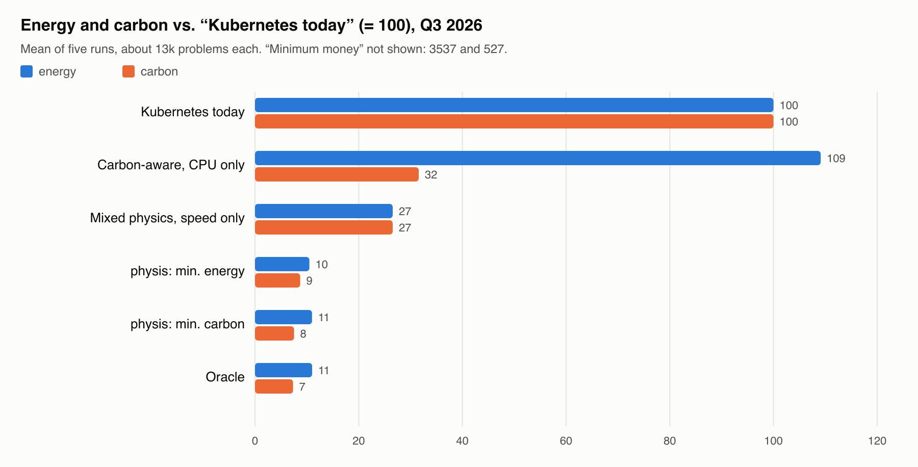
Energy and carbon of the seven policies relative to “Kubernetes today”, third quarter of 2026
The first quarter (winter) shows the same picture: “minimum energy” cuts energy by 89% and carbon by 91%, “minimum carbon” cuts carbon by 92%, the oracle also by 92%, and carbon-aware scheduling on CPUs alone cuts carbon by 69% at the cost of a 9% increase in energy.
Four conclusions follow from these numbers.
Choosing the physics matters more than choosing place and time combined. Shifting work in time and space on processors alone (what is now called carbon-aware scheduling) removes about 70% of the carbon, but adds 9% to energy and makes batch work wait almost three hours on average. Changing the physics alone, even without any energy goal, gives −73% on both metrics with no waiting. physis with an energy goal gives minus 90% energy and 91% carbon, also with no waiting. Waiting for clean hours adds another 14% of carbon savings on top.
Goals must be chosen deliberately: “minimum money” is a dangerous goal. Day-ahead markets sometimes have negative prices: the grid pays for consumption when there is nowhere to put a surplus of wind and solar. In the third quarter of 2026 this happened in 7.6% of quarter-hours in Germany, 6.5% in France and 3.7% in Poland (where the minimum reached −120 € per MWh). A scheduler that minimizes money picks the most energy-hungry option in those hours, the living neuron culture with its life support (3.6% of problems), and in total spends 35 times more energy than Kubernetes, literally earning money by doing so. From the standpoint of the price signal this is correct behavior, because the grid needs load; from the standpoint of carbon and common sense it is wrong. The design lesson is that money must never be the sole goal: a composite goal is needed, or an energy and carbon constraint on top of money. Mandates with a daily budget in joules and grams (principle P10) offer one way to do this.
The forecast is worth little. The oracle, which sees the future exactly, beats our naive “same as yesterday” forecast by only 2.5% of carbon in the third quarter and 2.6% in the first. Almost all of the gain comes from the choice of physics and from waiting as such, not from forecast accuracy.
Deadlines are practically never missed. The only miss across five runs came from the “minimum money” policy. A quality shortfall affects fewer than 1% of problems against a declared 90% lower confidence bound. For the physis policies it is slightly higher (0.9% versus 0.7%), because they more often pick the minimum effort that statistically still meets the target.
8.3. Data movement: computation should go to the data
In the first version of the simulator, the energy of moving data was charged at the carbon intensity of the destination country, and the scheduler eagerly shipped problems to France with its nuclear power, so that up to a third of the work moved there. This was a modeling error. Data travels over networks between countries, and it is more honest to charge the transfer at the average intensity of source and destination. After the fix, the only work physically moved was the work that sovereignty constraints forced to move, that is, 4.8% of problems. The scheduler did not move a single problem voluntarily.
The reason is scale. According to Aslan and coauthors, transferring data over core and fixed access networks cost 0.06 kWh per gigabyte in 2015 and halved roughly every two years [85]. Extrapolating to 2026 gives about 4.8 µJ per byte. The G22 graph weighs about 480 KB, and moving it costs on the order of 2.3 J. Solving the same problem on reversible logic costs 4 mJ, five hundred times less. The more economical the physics of computation becomes, the more data movement dominates the bill. This is the same pattern Mark Horowitz showed inside a chip, where a memory access costs orders of magnitude more than an arithmetic operation [36]. Only now it shows up at the scale of power grids and countries. We ran the experiment with data volumes from 65 bytes to 100 MB per image, and the share of voluntary transfers stayed at zero in every case.
We assumed intra-zone transfer to be ten times cheaper than inter-zone transfer, and that is an assumption. But the conclusion does not depend on it. In a world where computation gets cheaper by orders of magnitude while the network gets cheaper by half every two years, the scheduler should bring the computation to the data, not the other way around. For the design, this is an argument for data movement as an explicit, planned operation with a price (section 6) and against a flat network in which movement is invisible.
8.4. The model is wrong — the system learns
The most important question about emulation is what happens if the model of a real machine turns out to be wrong. We tested this directly. Five physics (digital annealing, SFQ, reversible logic, p-bits and photonics) consume 30 times more energy in the “world” than the scheduler’s model assumes. That is enough for trust in the model to lead to the wrong choice of physics. We compared three variants:
| Variant (Q3) | Energy, Wh | Carbon, g | Work on the “wrong” physics | Forecast error: first 10 runs → first 100 → end of quarter |
|---|---|---|---|---|
| No learning | 11.97 | 2.99 | 64.6% | 67% → 74% → 73% |
| Learning from receipts | 5.42 | 0.78 | 29.7% | 32% → 7.6% → 4.4% |
| Truth known in advance | 5.41 | 0.74 | 30.3% | 3% → 4.4% → 4.2% |
Without learning, the scheduler keeps trusting the model and spends 2.2 times more energy. With learning, the forecast error drops from 32% over the first ten runs to 7.6% over the first hundred and then settles at the noise level (about 4–5%). The resulting energy and share of work on the “wrong” physics practically match the variant in which the truth is known in advance. The first quarter gives the same numbers.
This is exactly why emulation in the prototype is not a sham but an experimental setup. The substrate model serves as a starting hypothesis, not a claim. On real hardware, the system will reconcile it with reality through receipts within the first few hundred runs.
Along the way, this experiment uncovered another bug. At first the learning did not converge and the error stayed around 60%, because receipts were compared against the already corrected forecast, so the system was learning a “correction to the correction.” Now the actual value is compared against the raw model prediction, without corrections, site overhead or data movement.
8.5. How much the conclusions depend on assumptions
Most parameters of the emulated physics are set by assumptions with ranges. One at a time, we moved each physics to the pessimistic end of its range (energy and power at maximum, speed at minimum) and to the optimistic end, changing both the “world” and the scheduler’s model simultaneously. We then looked at what share of work that physics receives and what happens to total carbon. Each point got three runs in both quarters; the third quarter is shown below, and the first leads to the same conclusions.
| Physics | Share of work (min. carbon): pessim. / nominal / optim. | Total carbon, g: pessim. / nominal / optim. |
|---|---|---|
| Reversible logic | 30.8% / 31.2% / 32.3% | 0.191 / 0.189 / 0.185 |
| p-bits | 6.2% / 8.7% / 8.9% | 0.192 / 0.189 / 0.189 |
| Photonics | 2.3% / 2.3% / 2.3% | 0.189 / 0.189 / 0.189 |
| Neuromorphic chip | 0% / 2.2% / 2.2% | 0.189 / 0.189 / 0.189 |
| Digital annealing | 0% / 8.6% / 13.7% | 0.349 / 0.189 / 0.146 |
| SFQ | 0% / 13.3% / 18.2% | 0.250 / 0.189 / 0.146 |
| Quantum processor, optical Ising machine, living culture, analog memory | 0% for any parameters | unchanged |
By this table, the physics fall into three groups.
- Robust. The shares of reversible logic, p-bits, photonics and the neuromorphic chip barely depend on where in the assumption range the truth lies.
- Assumption-dependent. The role of digital annealing and superconducting logic is determined entirely by their speed, power and, for SFQ, the cost of cooling. At the pessimistic end the scheduler stops choosing them, and total carbon rises by 32–84%. These physics need calibration on real hardware before any conclusions are drawn.
- Never chosen for these problems: the quantum processor (cryogenics eats everything on problems of up to 20 vertices), the optical Ising machine (both worse quality and higher energy), the living culture (slow and expensive because of life support) and analog memory (photonics solves the same classification more accurately and more cheaply). This is not a verdict on these physics but a property of these problems and these models, and it is precisely what the scheduler must be able to see.
The most important point for the whole article is that even at the most pessimistic end of any physics, the total carbon of physis is 84% lower than that of “Kubernetes today” (0.40 g versus 2.52 g in the third quarter, 0.47 g versus 2.95 g in the first). Sensitivity changes which special physics wins, but not the fact that choosing the physics wins.
That said, the physics were shifted one at a time rather than all at once, and the ranges are our own choice. A joint pessimistic scenario will be the next test.
Reproducibility. We reran all simulations from scratch in a build pod of the workshop cluster, that is, on an AMD EPYC 9454P server processor under Linux rather than on a laptop with an Apple M4 under macOS. With the same published calibration, the final tables of all four experiments for both quarters matched the published ones byte for byte, and in the summary files the numbers differed by less than one billionth, which is explained by different floating-point arithmetic on the two architectures. Then we did something the published numbers had not: we recalibrated all physics on the EPYC itself (9429 records, results/repro/) and repeated the main experiment. The server processor runs our problems more slowly than the M4, so the “Kubernetes today” baseline became roughly one and a half times more expensive in energy, while the physis policies barely changed. As a result, the advantage grew: in the third quarter, physis with an energy goal cuts energy by 93% and carbon by 94%, versus 90% and 91% in the published version. This is the very inaccuracy mentioned in the limitations: the M4’s speed combined with the EPYC’s power made the processor in the simulation slightly more favorable than it really is, which means the published numbers are more conservative than calibration on a real server processor implies.
8.6. Live testbeds

A live testbed: Kubernetes without nodes and twenty substrates. The same problem at quality targets of 0.95, 0.99 and 1.0 goes to hyperdimensional computing, to int8 compute in memory and to an exact GPU, followed by a real run and a signed receipt that passes verification.
The recording was made by the hack/demo.sh script on the node-free testbed; everything it shows is live kubectl output.
A real-time stream of 120 problems (MaxCut on Gset and random graphs, digit classification, four different policies, a third of the problems restricted to “EU only”) ran on both testbeds against fresh power grid forecasts for November 8, 2026. The random number generator starts from the same seed, so the sequence of problems is identical and the testbeds can be compared. On the node-free control plane:
- all 120 problems completed, with no missed deadlines;
- the work spread across five physics: reversible logic took 47 problems, photonics 27, CPU 26, p-bits 12, SFQ 8;
- quality fell short of the target in 3 cases out of 120 (2.5%), which is within the stated 90 percent confidence;
- the median time from problem creation to an agent claiming it is 2.3 s, and the 95th percentile is 3.7 s. This is the cost of polling: the scheduler checks problems every 2 seconds and the agent once a second;
- all 120 receipts from the run, in six chains, were verified with the substrates’ public keys without any access to the system.
On kuberoot, where physis runs as pods:
- all 120 problems completed with no missed deadlines, and the split across physics was the same: reversible logic 47, photonics 27, CPU 26, p-bits 12, SFQ 8. Given the same input, the scheduler makes the same decisions wherever it runs;
- quality shortfalls: 3 out of 120;
- work claim latency: 2.4 s at the median, 3.6 s at the 95th percentile;
- after the run, all 132 receipts in 7 chains were verified with the substrates’ public keys, and a tampered copy was rejected;
- deferred work is visible live: in test TC-09 the scheduler placed a flexible problem with a one-day deadline 18–19 hours later, at noon the next day, when the forecast had the French grid at 63 g CO₂ per kWh.
Kuberoot also found a bug that the node-free testbed missed. The random number generator seed is stored in the receipt as a 64-bit integer, but when the object was converted for the API it passed through a floating-point number and lost its low-order digits. The signature covered the exact value, while the stored value was rounded. On kuberoot, test TC-10 correctly rejected such a receipt. Numbers are now passed exactly, and a unit test checks that a receipt makes a round trip through the API without a single change.
A second real physics: GPU. On the node-free testbed, a fifteenth agent, gpu-m4, joined the 14 others. It sends classification to the Apple M4 GPU through MLX (tools/gpu-worker.py) and measures time on the GPU itself, separating the preparation of Metal compute kernels (the programs that run on the GPU) from the computation. Calibration over 21 batches gave quality equal to the exact classifier (float32 changes no answers), throughput from 8·10⁸ multiply-accumulates per second on a batch of 1797 images to 6.5·10⁹ on a synthetic batch of 200,000, and a preparation time of 3–14 ms (about 50 ms when the compiled kernels are not yet cached; measured separately in hack/gpu-benchmark.py, results/gpu-throughput-benchmark.txt). Conformance on the testbed with the GPU is 17 out of 17.
We then ran the same batches on a real CPU and a real GPU, five times each (results/real-cpu-vs-gpu.json, medians):
| Batch | CPU, time | CPU, energy | GPU, time | GPU, energy |
|---|---|---|---|---|
| 100 images | 0.14 ms | 0.8 mJ | 5.5 ms | 44 mJ |
| 500 | 0.29 ms | 1.7 mJ | 6.0 ms | 48 mJ |
| 1797 | 1.1 ms | 6.9 mJ | 6.7 ms | 53 mJ |
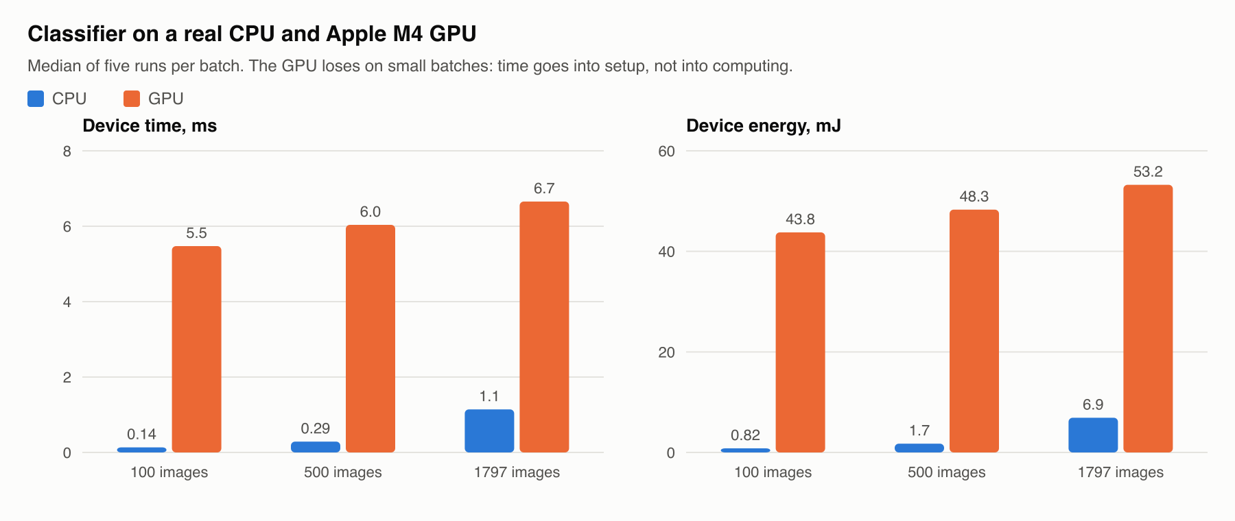
Time and energy of a real CPU and a real Apple M4 GPU on batches of 100, 500 and 1797 images.
On batches like these the GPU loses to the CPU by 6–40 times in time and by 8 to more than 50 times in energy, because preparation, not computation, eats everything. Energy here is the measured time multiplied by a model power, which for the CPU is taken as a fraction of the rated power (TDP) of a server EPYC and for the GPU is assumed. At the measured speeds, the times would break even at roughly 12 thousand images and the energy later, and exactly where depends on the GPU’s power, which we do not yet measure. Without corrections from receipts, the scheduler is wrong whenever the models are. At a target of 1.0 it picks the GPU (this is visible in the testbed recording above), even though the real CPU is eight times more economical on that batch. The same experiment shows why receipts are needed. The CPU model with its initial, uncalibrated speed overestimated time by 9–22 times, and the GPU model underestimated it by a third; the scheduler corrects both from receipts (section 8.4).
Kubernetes without containers and without nodes. The last testbed was a kuberoot node from the physis distribution, built in the workshop cluster and booted in a virtual machine on one of that cluster’s servers. It runs only operating system services: the kine store (an etcd replacement on top of an ordinary database), the API server, the controller manager, the kuberoot node API, the physis scheduler and the substrate agents — twelve at first, and in the latest build all twenty emulated ones. kubectl get nodes and kubectl get pods -A return nothing, because this cluster has no Node objects and no pods, and the node has no containerd or kubelet. The conformance suite passes 17 out of 17 with both twelve substrates and all twenty (results/containerless-node*.txt, results/conformance-kuberoot-containerless-*.json). The first build, with eight substrates, gave 15 out of 17: TC-13 temporarily silences one substrate, which left only one physics for MaxCut, and TC-14 had no slow substrate to cut off mid-work. This is a requirement on the set of substrates, not on the core, and with twelve substrates the tests pass. During boot the agents restart twice while the API server comes up, so the order of services in the profile could be refined.
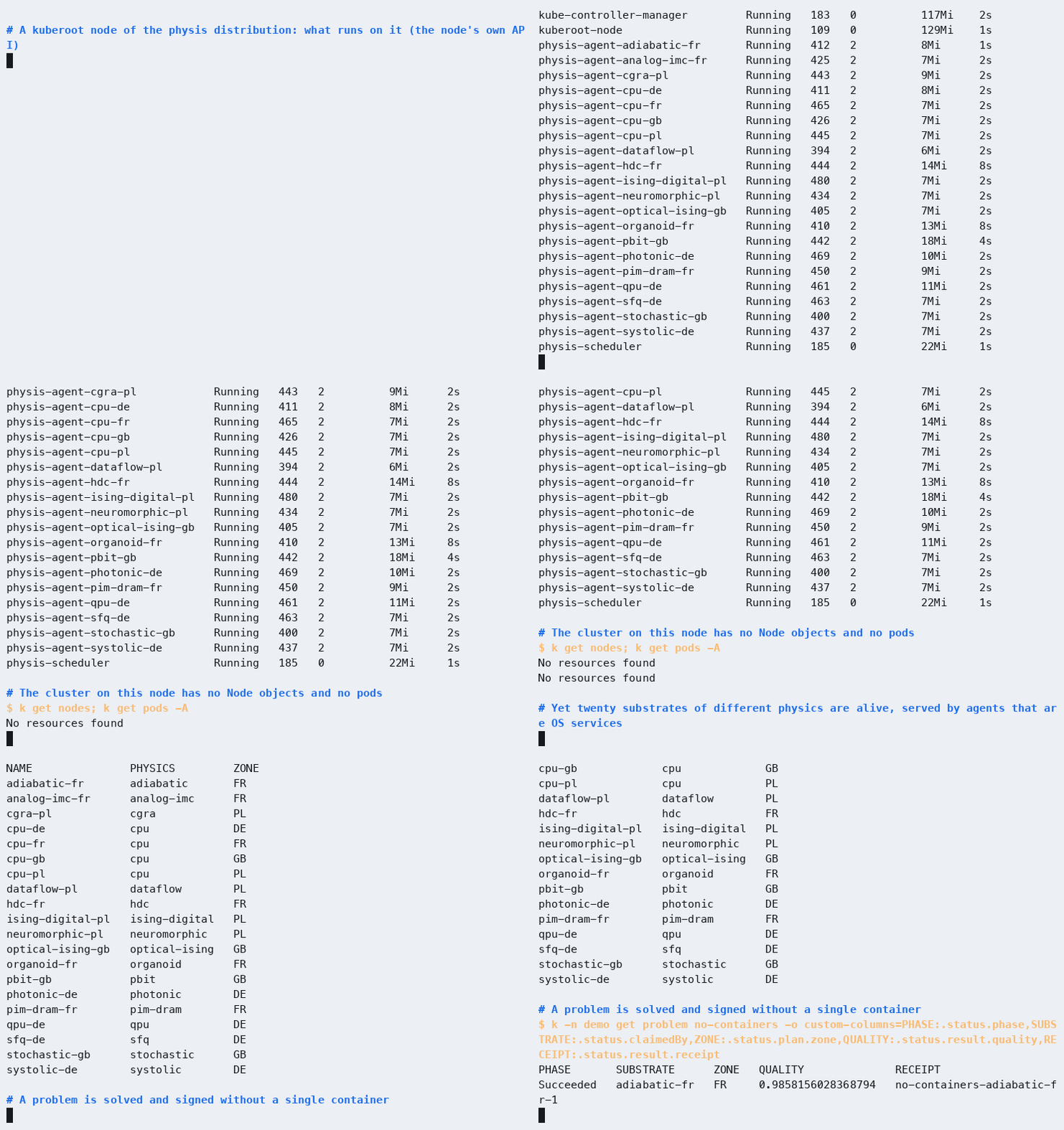
A kuberoot node without containers: only operating system services, empty node and pod lists, twenty substrates and a solved problem.
A bridge from DRA. On the testbed we published a ResourceSlice with one device, the laptop’s Apple M4 GPU, for which the driver specified speed and preparation time but said nothing about power. physis-dra-bridge created the substrate dra-m4-gpu0, whose model labels speed and preparation with a reference to the driver and power and preparation energy as assumptions. An agent with the -adopt flag took it over without changing its description and solved a classification problem on the real GPU (results/dra-bridged-*.json). We repeated the same on a four-node kuberoot cluster: the device cpu.example.com/rack-7/cpu0, for which the driver specified only power, became a substrate, an agent pod took it over, and a problem allowed only in the CH jurisdiction went to it (results/dra-cluster-*.json).
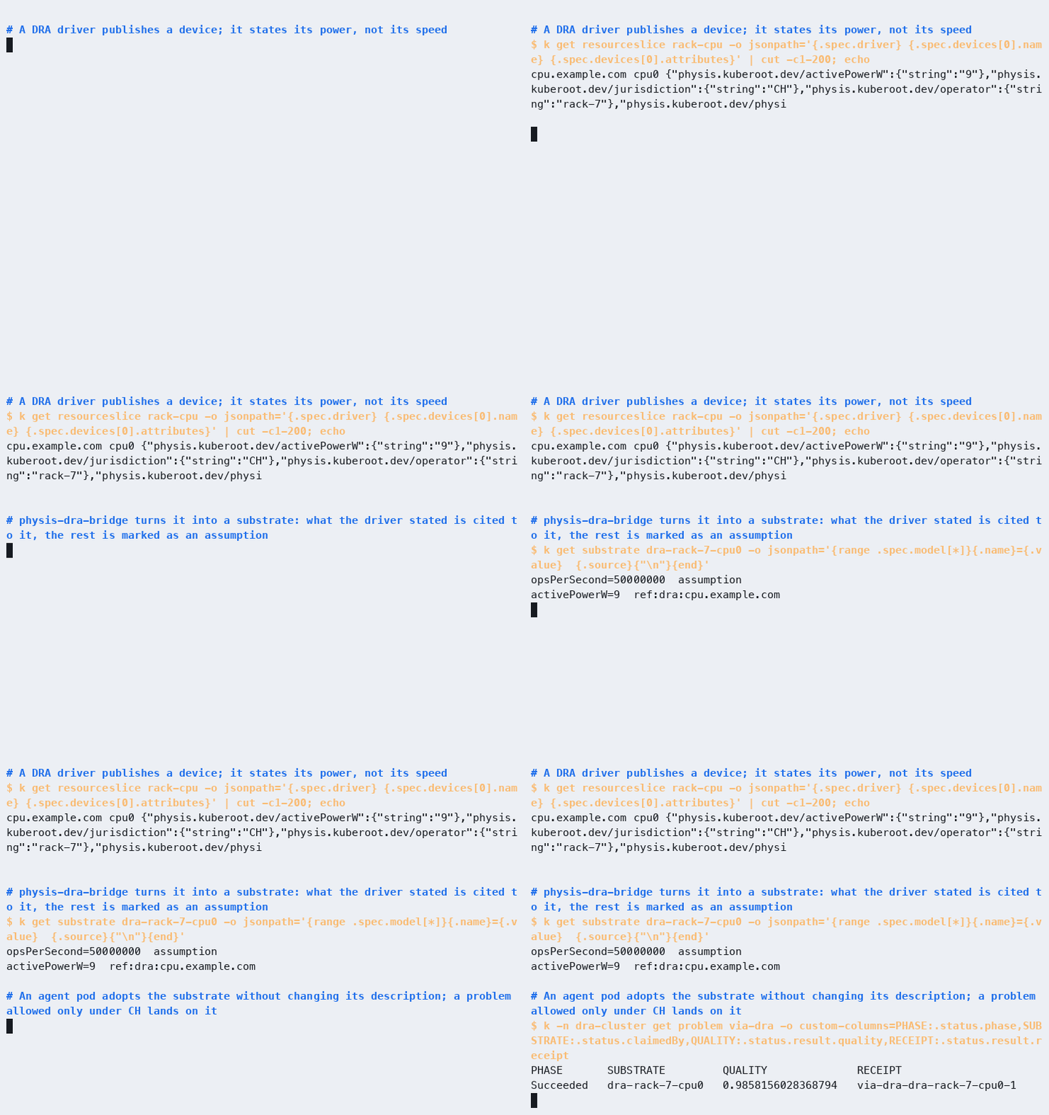
A bridge from DRA on a kuberoot cluster: a device from a ResourceSlice, a substrate model with parameter provenance, and a solved problem.
Scheduling hierarchy. We replaced the single scheduler with a global one and two site schedulers, for DE and FR, and submitted a stream of 12 problems allowed in all four zones. The global level chose the FR zone and handed the problems to that site, which picked the substrate, and all 12 were scheduled by the FR site. We then stopped the global level and submitted another 12 problems, six allowed only in DE and six anywhere. Without the global level, the DE site scheduled all six problems in its zone on its own, and the FR site picked up the problems with no zone restriction. There was no rescheduling and no double execution, because the API’s optimistic locking separates two sites that take on the same problem (results/hierarchy-problems.json).
On the kuberoot cluster, where the levels run as pods, the first run showed a mixed picture: the global level scheduled some problems itself, and the sites took others while the global level was still alive. There were two causes. The API server rejected every lease renewal because the time in it was written with nanoseconds while the field accepts only microseconds; in addition, the lease was renewed at the start of the scheduling cycle, and on a CPU-limited pod the cycle ran longer than allowed. The lease is now renewed on its own timer and in the correct format, and a level’s freshness is judged the same way as in leader election in client-go, the standard Kubernetes client library: by whether the lease value changes, not by comparing someone else’s clock with one’s own. After the fix, everything on the cluster went as on the testbed: the global level handed all 12 problems to the FR site, and without the global level the sites scheduled their own problems (results/hierarchy-cluster-*).

Scheduling hierarchy on a kuberoot cluster: leases of three levels, problems routed through the FR site, and after the global level stops, DE problems scheduled by the DE site.
The device core in a WASI sandbox. The wasi-cpu-ch agent on the testbed neither computes nor signs anything itself; that is done for it by physis-device, built for WebAssembly and run in wasmtime with access only to its own state directory and to the data. The signing key was generated inside the sandbox and never leaves it. Five MaxCut problems on graph G1 were solved with quality 0.994–0.996, and the receipts are signed with the key from the sandbox and pass chain verification (TC-10) (results/wasi-device-*.json). Along the way, this experiment uncovered a bug in the newly added local level, where the agent took its own lock twice and froze after the first result. It was fixed before publication.
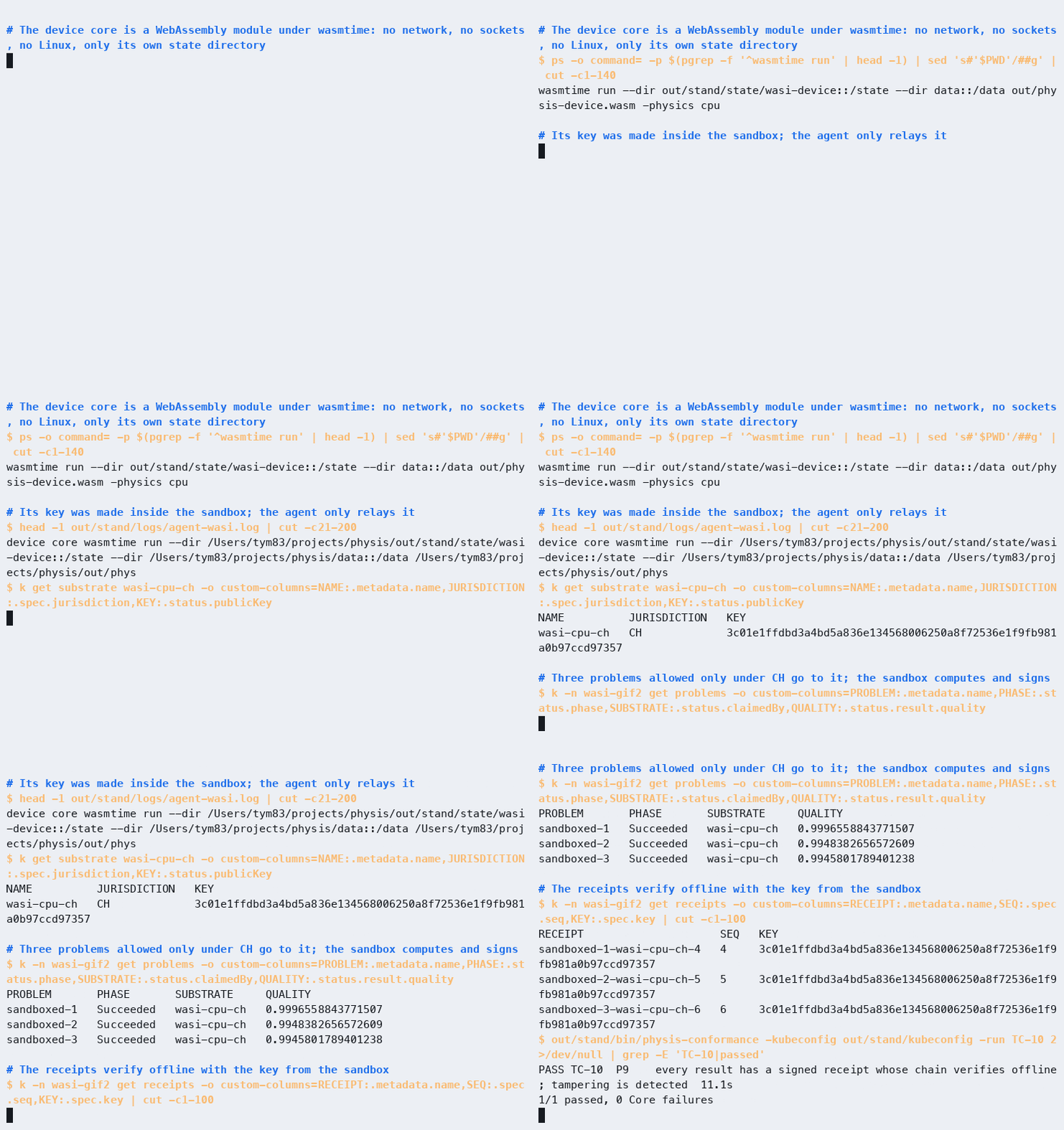
The device core in a WASI sandbox: wasmtime with access only to its own directory, a key generated in the sandbox, solved problems and receipt chain verification.
MCP for agents. On the live testbed and then on the kuberoot cluster, the plan tool from physis-mcp returned a dry-run plan with alternatives and machine-readable reasons, submit with a requestID created a problem, and a repeated submit with the same requestID returned the existing problem instead of creating a second one (results/mcp-cluster.jsonl). An infeasible request is rejected with the code QualityUnreachable, from which the agent can decide what to do next.

MCP from the agent’s side: a dry-run plan, submission with a request ID, a retry that does not start a second run, and a rejection with a code.
Five architectures that change how computation is done. Five substrates were added to the testbed: a systolic tensor array (modeled on the TPU), compute in DRAM (HBM-PIM), a dataflow processor (Groq), and stochastic and hyperdimensional computing. Their emulators faithfully do what the hardware would do: they quantize weights and inputs to FP8 or FP4 with block scaling, compute in int8 with 32-bit accumulation, encode numbers as random bit streams, and build and train hypervectors. As a result, answer quality is measured rather than assumed. Time and energy come from device models with sources: the peak speed of TPU v1 and its power [26], the peak speed of Groq [28] (its power is an assumption, since the sources do not give it), the speed of HBM-PIM [31] with energy derived from the cost of a DRAM read [36] and the PIM gain [32], and assumptions with ranges for the stochastic and hyperdimensional schemes. Calibration produced 3024 records (results/calibration-numeric-runs.csv). Results on a batch of 1797 images (quality as a fraction of the exact classifier):
| Substrate | Variant | Quality | Energy per batch |
|---|---|---|---|
| Tensor array | int8 | 1.000 | 40 mJ |
| Tensor array | FP8 (E4M3) | 0.999 | 40 mJ |
| Tensor array | MXFP4 (E2M1) | 0.984 | 40 mJ |
| Compute in DRAM | int8 | 1.000 | 53 µJ |
| Dataflow | int8 | 1.000 | 30 mJ |
| Stochastic | 64-bit stream | 0.975 | 0.37 µJ |
| Stochastic | 1024-bit stream | 0.998 | 5.9 µJ |
| Hyperdimensional | 512 dimensions | 0.964 | 0.04 µJ |
| Hyperdimensional | 2048 dimensions | 1.007 | 0.16 µJ |
Three conclusions follow from the table. Reduced precision costs almost nothing in quality: FP8 loses one thousandth, int8 loses nothing, and FP4 loses one and a half percent. Stochastic and hyperdimensional schemes buy quality with stream length and dimensionality, exactly as annealing buys it with steps. And on small batches the tensor array and the dataflow processor lose to compute in memory, because their energy goes into preparation and the power of a whole card rather than into multiplications (for the same reason, the three tensor array variants cost the same).
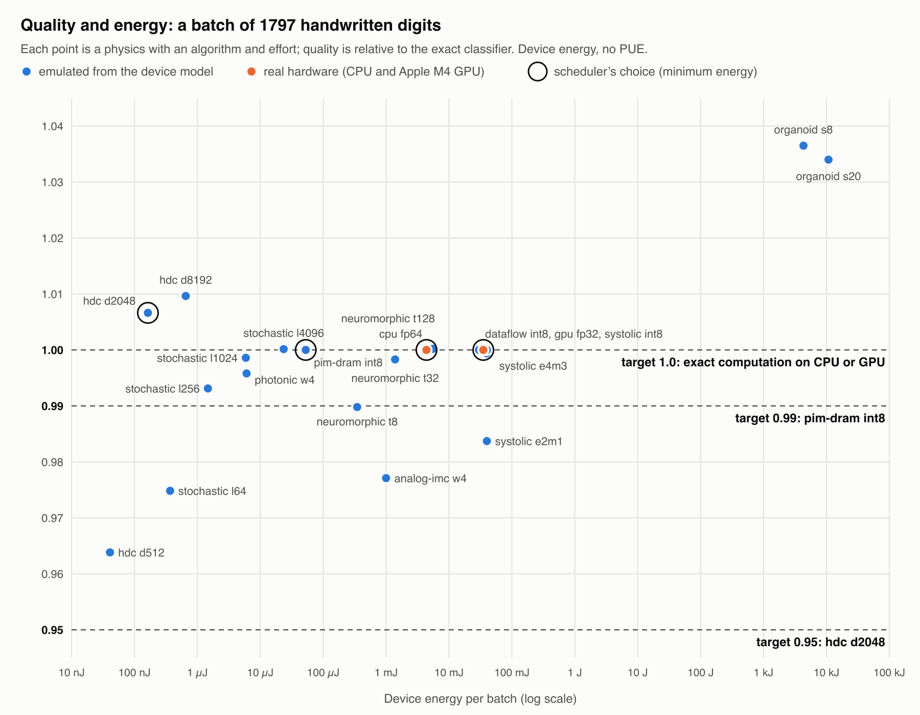
Quality versus energy on a batch of 1797 images for all classifiers. The scheduler’s choices at targets of 0.95, 0.99 and 1.0 are circled.
The main point, though, is that the choice depends on the required quality. We asked the scheduler about a batch of 1797 images (dry-run plan, minimum energy). At a target of 0.95 it takes hyperdimensional computing with 2048 dimensions (about 0.2 µJ including PUE); at 0.99 those no longer pass on confidence, and the scheduler moves to int8 in memory (64 µJ); and at 1.0 only exact computation on the CPU and GPU remains. With the “fastest” policy, the dataflow processor wins at targets of 0.95 and 0.99. Conformance on the testbed with all 20 substrates is 17 out of 17.
The last addition was a reconfigurable CGRA fabric with Plasticine parameters, that is, 12.3 TFLOP/s at no more than 49 W [40], where the lower bound on speed accounts for real applications achieving 18–25% of peak performance. It runs the same annealing and exact classifier as the processor, so its quality is the same, and what differs is speed and energy. Calibration produced 669 records (results/calibration-cgra-runs.csv). With it the testbed has 21 substrates, conformance again gives 17 out of 17, and the fabric immediately shows up on the trade-off frontier. In dry-run plans with the “fastest” policy it beats reversible logic and p-bits on MaxCut on graph G22, and in classification it sits alongside compute in memory and the dataflow processor.
A two-machine kuberoot cluster and a real network partition. The third testbed consists of two kuberoot edge virtual machines from the same boot media. Each has two network interfaces, one for external access and the other for a direct link between the machines, with addresses 10.0.0.11 and 10.0.0.12. The first machine serves as the control plane node, and the second joined the cluster as a worker node with a one-time invitation (JoinTicket). The agents are split evenly across the machines, seven and seven, by a scheduling constraint in the Helm chart; the scheduler is pinned to the control plane node. The conformance suite on this cluster passes 17 out of 17.
Above all, the second node makes it possible to test a partition at the network level rather than through an annotation. A privileged pod on the worker node takes down its cluster network interface and brings it back up after a set time. The agents on the worker node lose contact with the API server entirely, including heartbeats, work claims and reports.
- A stream during the partition. A stream of 120 problems, with the worker node losing connectivity for two minutes at second 90. All 120 problems completed. During the partition, the control plane node’s substrates claimed 41 problems and the cut-off node’s substrates none. No problem got stuck on a silent substrate, because the scheduler stopped offering those substrates as soon as their heartbeat went stale. Once connectivity returned, the worker node’s agents started claiming work again.
- Work claimed before the partition. The living culture agent was moved to the worker node and given a batch of 100 images, and as soon as it claimed the batch, connectivity dropped for 90 seconds. The work finished 11 seconds after the claim, already without connectivity. The report with a signed receipt arrived 2 seconds after connectivity returned.
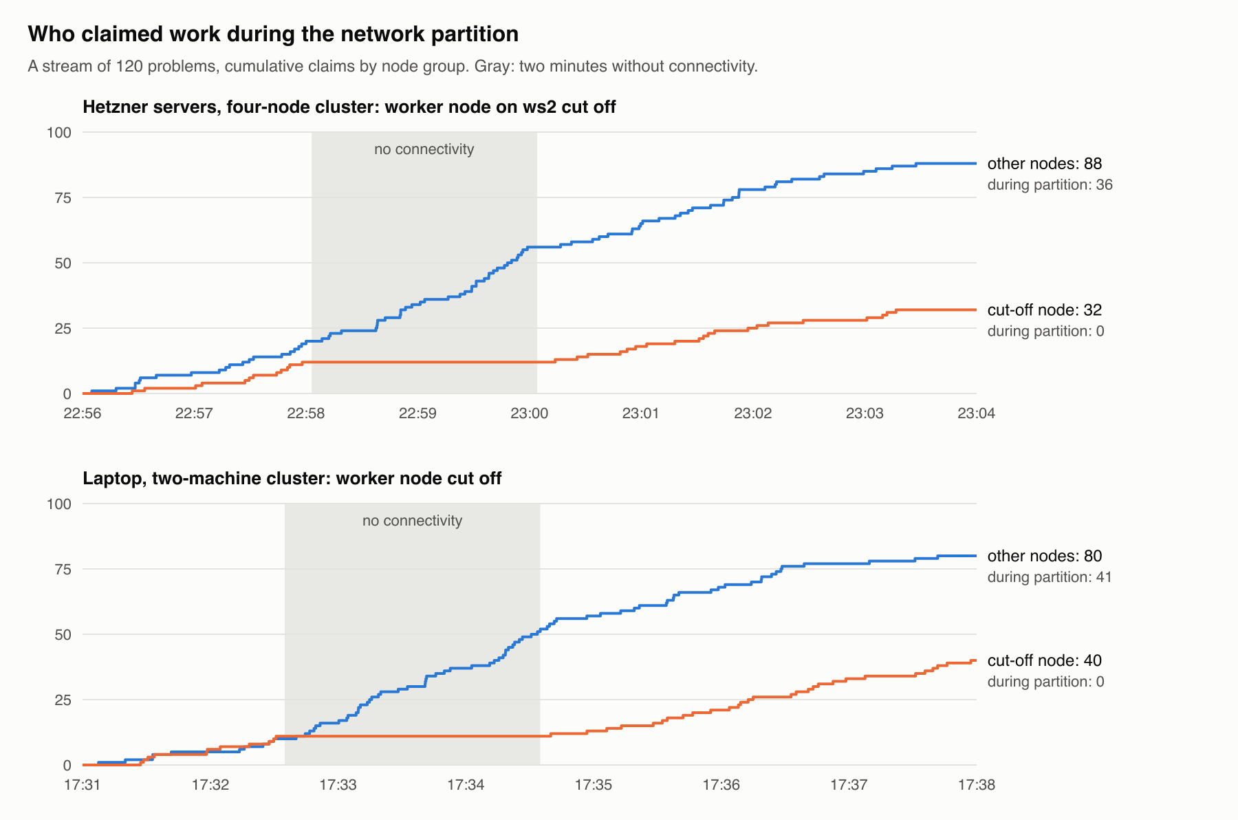
Problem claims over time: while the worker node is cut off, only the other nodes claim work.

A real-time network partition on a kuberoot cluster: the cut-off node’s problem counter stalls while the other nodes claim work, and once connectivity returns the node takes problems again. All 60 problems completed.
Our testbed turned up three more bugs. The first, a serious one, was in the prototype: the agent kept its signing key in the pod’s temporary directory. After a restart it came back with a new key, silently replaced the published one, and its earlier receipts stopped verifying. TC-10 caught this after the agents were restarted. The key is now stored in a Secret and survives agent restarts and moves, and if the key does change, the old one stays on the substrate’s list of previous, retired keys. Earlier receipts are verified against it, and a receipt signed with a key the substrate never published is rejected. After the fix we restarted all 14 agents, and the keys did not change. The second bug was in the test suite itself, where TC-14 set an annotation based on a stale read of the object and conflicted with the agent’s heartbeat. It now retries the write on conflict. A third was in the packaging: the Helm chart shipped an old copy of the calibration, without the GPU, the new architectures and the CGRA, so on the cluster these substrates were alive but the scheduler never chose them, and conformance did not notice. The chart now takes the calibration from results/, and a test fails if the copies diverge; after the fix, the scheduler on the cluster picks the same physics as on the testbed.
This is what TC-13 and TC-14 check with an annotation, but now on a real network partition. The data is in results/partition-* and results/conformance-kuberoot-*.json, and the scripts are in hack/kuberoot-local-multi.sh and hack/kuberoot-partition-*.sh.
8.7. The environments where we tested all of this
| Environment | What was tested on it |
|---|---|
| Apple M4 laptop (macOS, arm64) | Calibration: 6405 records across all algorithms on all physics; unit tests (25 tests: solvers against exhaustive search, scheduler, receipts, mandates, receipt round trip through the API) |
| Control plane without nodes: kube-apiserver 1.37 and etcd from envtest, 14 agents as processes | End-to-end operation without Node objects; live stream of 120 problems; conformance 17/17 and a control run at 0/17 |
| Digital twin on DE, FR, PL, GB power grid data for the first and third quarters of 2026 | Comparison of seven policies, value of forecasts, data transfer, learning under a wrong model, sensitivity to assumptions |
kuberoot edge cluster: built from source for arm64, booted in QEMU (HVF) on macOS, single-node cluster on Kubernetes 1.37.1; physis as pods from the kubepkg package’s Helm chart, applied with kubectl | conformance 17/17; live stream of 120 problems; verification of all receipts afterwards; found and fixed a numeric precision bug in receipts |
| Two-machine kuberoot cluster: the same boot media with static cluster network addresses, worker node joined via JoinTicket; agents 7 + 7 | conformance 17/17; stream of 120 problems with a two-minute network partition of the worker node; work claimed before the partition and reported after it |
| kuberoot cluster in a tenant of the Cozystack workshop cluster (KubeVirt on Hetzner servers), amd64, built in the cluster: first three nodes (one on server ws1, two on ws3), then four (plus ws2) | conformance 17/17 on three and on four nodes; streams of 120 problems with a two-minute network partition of the worker node on ws3 (three nodes) and on ws2 (four nodes); work claimed before the partition and reported after it (three nodes); found and fixed the agent key bug and the concurrent write conflict in TC-14 |
kuberoot node without containers (physis distribution): a KubeVirt virtual machine on a workshop cluster server, physis as operating system services, no Nodes or pods | conformance 17/17 with 12 and with 20 substrates |
Four-node kuberoot cluster on the current codebase: 20 substrates, calibration from results/ | conformance 17/17; level hierarchy as pods; bridge from DRA; identity-based handoff between nodes; MCP; real-time network partition |
9. Conformance for tomorrow’s systems
Kubernetes conformance answers the question “does the cluster implement the API the same way the reference does.” Our suite asks a different question: does the system behave the way the principles require. It is a black-box suite: it talks only to the API, creates problems in its own namespace, and judges by behavior rather than by internals. Any implementation of the physis.kuberoot.dev/v1alpha1 resources can pass it, not just ours. The full specification is in docs/conformance.md.
The tests come in two levels. The base level, Core, is mandatory. The extended level, Extended, is expected of production systems and may be skipped with a stated reason. A skip never counts as a pass.
| Test | Level | Principle | Requirement |
|---|---|---|---|
| TC-01 | Core | P3 | Every live substrate declares its physics, zone, operator jurisdiction, and a model in which every parameter has provenance |
| TC-02 | Core | P7 | Work runs without Node objects, and the system’s roles grant no access to nodes or pods |
| TC-03 | Core | P2, P4 | A result request is scheduled with a forecast of time, energy, and grid carbon intensity, and completes by its deadline |
| TC-04 | Core | P4 | The plan shows alternatives, and none of them is worse than another on every metric at once |
| TC-05 | Core | P5 | An unachievable result is rejected with reasons and is never started |
| TC-06 | Core | P4 | The budget is a hard limit |
| TC-07 | Core | P11 | Allowed zones and operator jurisdictions are hard constraints |
| TC-08 | Core | P14 | A dry-run plan request returns a plan and starts nothing |
| TC-09 | Extended | P12 | Flexible work with a long deadline is placed at the minimum forecast carbon among the alternatives |
| TC-10 | Core | P9 | Every result has a signed receipt; the chain is verifiable without access to the system; tampering is detected |
| TC-11 | Core | P9 | Receipts cannot be modified |
| TC-12 | Core | P10 | Work under a mandate with a foreign signature is rejected; a plan above the threshold waits for human approval and runs after it |
| TC-13 | Core | P7 | Work scheduled onto a substrate that has gone silent returns to the pool and runs on another one |
| TC-14 | Extended | P8 | A substrate cut off from the API after claiming work finishes it and reports the result once connectivity returns |
| TC-15 | Core | P2, P3 | The same class of problems can run on more than one physics |
| TC-16 | Core | P5 | The result reports the quality achieved; the plan reports a lower confidence bound and the number of observations behind it |
| TC-17 | Core | P11 | Data transfer is estimated from Link objects; paths through forbidden jurisdictions are not used |
TC-13 and TC-14 require making a substrate unreachable. In a real installation this is done with a network policy; the reference suite uses a portable technique instead, the physis.kuberoot.dev/simulate-partition-until annotation on the substrate. When the agent sees it, it stops all communication with the API until the specified time but does not interrupt work already in progress.
Results
physis passes 17 of 17 on five testbeds: a control plane with no nodes at all, a single-node kuberoot cluster, a kuberoot cluster of two virtual machines on a laptop, a four-node kuberoot cluster on three physical servers, and a kuberoot node with no containers at all, where physis runs as OS services.
A control run on the same control plane with the same CRDs but without the scheduler and agents — roughly what plain Kubernetes provides — scored 0 of 17. We needed the control run to check the tests themselves, and it found a bug in them. With no substrates present, TC-07 checked nothing and was counted as passed. The test now requires that there be something to check: live substrates in at least two zones and two jurisdictions.
The suite also found five real bugs in the prototype before we knew about them. First, an unknown price was stored as NaN (the special “not a number” value), which cannot be serialized to JSON, so plans were simply not written. Second (TC-04), with an unknown price every comparison with NaN is false, so options that were worse than others on every metric ended up on the trade-off frontier. The correct approach is to treat options as incomparable on cost where the price is unknown and decide on the remaining axes. Third, the receipts lost precision in the 64-bit random generator seed, as described above; this showed up only on kuberoot. Fourth, the agent had a race condition, where the outcome depends on the order of concurrent writes: the agent’s heartbeat overwrote the substrate’s metadata from a slightly stale snapshot and could erase an annotation the operator had just set. Fifth, the agent’s signing key was lost on restart (section 8.6). The suite also turned up two bugs in the tests themselves. TC-14 compared timestamps with nanosecond precision while the annotation carries them with one-second precision, so the test occasionally failed spuriously; it also set the annotation based on a stale read of the object and conflicted with the agent’s heartbeat. Findings like these are exactly what conformance is for.
10. Limitations
This is part of the results, not an appendix to them. The full list is in docs/limitations.md.
- Sixteen of the eighteen physics are emulated. The real ones are CPU and GPU (an Apple M4 on the laptop testbed). For the GPU, time is measured while power is assumed, because Apple does not publish it. Conclusions that rest on a single assumed number should not be treated as conclusions; the sensitivity analysis shows which of them survive across the ranges.
- The same annealing run on CPU, digital, superconducting, and reversible devices yields identical quality by construction. Real hardware differs in precision and noise.
- The quantum processor emulation is coarse: fixed QAOA angles, up to 20 qubits, a global error model.
- The living culture is an echo state network with assumed noise.
- CPU energy is modeled. Measured CPU time is multiplied by a fraction of the TDP of a single EPYC 9454P core. The processor energy counters (RAPL) are not accessible inside the cluster’s pods.
- Calibration was done on a laptop (Apple M4). CPU speed in the simulator comes from the M4, while power comes from the EPYC.
- We compute carbon intensity for Germany, France, and Poland ourselves, without accounting for imports and exports, and lignite is treated as hard coal, which understates German intensity.
- Learning in the running scheduler is held in memory and lost on restart; in the simulator it persists. Within the conformance suite itself, the substrate outage in TC-13 and TC-14 is simulated with an annotation; a real network partition was verified in separate experiments on two-machine kuberoot clusters on the laptop and on the workshop cluster servers (section 8.6).
- The five architectures added later (tensor array, processing in DRAM, dataflow, stochastic, and hyperdimensional) run on the live testbeds and in conformance, but not in the quarter-long simulations, which were run earlier. Their quality is measured and their energy is modeled from peak rates; the power of the dataflow card and the energy per bit operation of the stochastic and hyperdimensional circuits are given as assumptions with ranges.
- The problems are small: they are measured in joules, not kilowatt-hours. What matters are the ratios, not the absolute totals.
- The workload is synthetic, with explicitly stated distributions.
- The kuberoot testbeds are virtual machines: in QEMU on the laptop (one node and two) and in KubeVirt on the workshop cluster servers (four nodes on three physical servers), not dedicated racks in a data center. The fault tolerance of kuberoot itself (multiple control planes, etcd) was not tested here. What was tested is that physis installs into kuberoot the standard way and behaves as the tests require.
- The network of tomorrow is only partly built. Links as objects with cost, transfer time, and path jurisdiction work and are checked by TC-17; identity-based substrate addressing with mutual authentication and object transfer between substrates work and have been verified by tests and on a testbed, but are off by default. A mailbox on API objects for substrates behind NAT, data transfer as a plan step, content addressing, and context-based transport selection remain design; a substrate’s jurisdiction is declared, not attested. Energy and bandwidth values for links come from Aslan’s estimate with extrapolation and from our own assumptions.
11. What comes next
physis is not a product but a claim tested in code. Some of what was on this list in the first version of the article is already done: a real GPU as a substrate, identity-based addressing, three levels of scheduling, a bridge from DRA, a device kernel outside Linux, and an interface for agents. The next steps suggest themselves:
- Real non-standard hardware. A cloud quantum processor, FPGA annealing, a neuromorphic board, servers with exposed energy counters, and then recalibrating the models from receipts on live data.
- Data transfer as a plan step, with content addressing and a mailbox on API objects for substrates behind NAT.
- A hierarchy without a central etcd. Today the levels share one store; the next step is giving sites their own stores and reconciling through receipts.
- A standard. Discuss the resources, the conformance profile, and the cost attributes in DRA with the community, the way CNI and CSI were once discussed (more in sections 12 and 13).
Everything is open: the code, the data (via download scripts), the tests, the models, and their sources. If the idea of infrastructure that aims at tomorrow rather than dragging yesterday along appeals to you, join in — with a substrate, with a critique of the model, or with a test our prototype will fail.
12. How to evolve Kubernetes so it serves both yesterday’s world and tomorrow’s
The simple conclusion from the prototype is that Kubernetes does not need to be rewritten; it needs a different boundary between the core and what plugs into it. Today the boundary is drawn as if a Linux machine and containers were part of the API itself. The Node object, the kubelet, the Pod, and the pod network are baked into the model, and anything unusual has to pretend to be one of them. Tomorrow a Linux machine will be one substrate among many, and the core should know no more about it than about a quantum processor.
What to keep in the core. The API server with its storage, watch, and optimistic concurrency; CRDs; RBAC; admission and audit; the “desired state plus controllers” model. This is Kubernetes’ real contribution, and the prototype relies on nothing else. On a testbed with no nodes at all, physis passes all 17 tests. The core is worth stabilizing as a product in its own right — a node-free control plane, which kcp has long been moving toward — with its own conformance profile that requires neither Node nor Pod.
What to make pluggable. Every place where a specific world is hard-wired today becomes a common interface with several implementations, just as CNI, CSI, and CRI once factored out networking, storage, and the runtime.
- Executor. The kubelet becomes one implementation of the substrate agent interface: describe itself with a model whose parameters carry provenance, report regularly that it is alive, claim work, sign the result, and deliver the report after a disconnect. A container node implements it through pods, a quantum processor through its control stack, a microcontroller through a device kernel on a serial port. The Node object remains for those who need it but stops being mandatory for every kind of work.
- Resource description. DRA already describes devices with structured attributes, but it lacks standard cost attributes (speed, energy per operation, power, setup, calibration windows) with provenance. This is a small extension that could be proposed as a KEP, the formal Kubernetes enhancement proposal, and the bridge in the prototype shows how it would map onto scheduling.
- Scheduling. Next to kube-scheduler, which places pods on nodes, we need a result scheduler as a separate pluggable component that works with problems described as results and with goals for energy, carbon, money, and jurisdiction. The kube-scheduler plugin mechanism (the scheduling framework) does not help here, because it answers the question “which node,” while the question is now “which algorithm, on which physics, where, and when.”
- Networking. kube-proxy and CNI become a detail of a single site. Between sites, the common interface becomes links as objects with cost and path jurisdiction, plus identity-based addressing, as in section 6.
- Accounting and trust. Signed receipts become a standard API alongside Events, immutable and verifiable without access to the cluster. Quotas gain dimensions in joules, grams of CO₂, and money, and mandates extend RBAC with budget delegation from a human to an agent.
How not to break the old world. Pod, Deployment, and Job stay. For existing work, a result problem can simply expand into a pod on the “Linux processes” substrate, so existing charts, operators, and GitOps keep working. The new pieces appear alongside, as CRDs and separate components, and displace the old ones only where they are better. That is how the prototype was built, and not a single step required changing Kubernetes code in the project’s main repository.
In what order. First comes what breaks nothing: standard cost attributes in DRA and energy accounting in metrics and quotas. Then the substrate agent interface as a separate specification and the result scheduler as an external component. Then a “tomorrow” conformance profile alongside the current one, so implementations can state honestly what they support. Only after that can Node and Pod become optional in the core, once there are live implementations for it and not just a prototype.
13. Cozystack as a platform for this layer
Cozystack is an open-source CNCF platform on which providers build their own clouds: Kubernetes, virtual machines on KubeVirt, managed databases, and clusters for tenants. None of what this article describes exists in it today. But structurally it is closer to the required shape than bare Kubernetes, because it already has tenants as a boundary of responsibility, a service catalog, providers across different sites, and GPU support. To become the foundation of the layer of tomorrow, it needs to go through several steps, and each one makes sense on its own.
The first step makes the tenant the holder of mandates and budgets. Today a tenant gets quotas for CPU and memory. It needs budgets in joules, grams of CO₂, and money, along with zones and jurisdictions, and the people inside a tenant need a way to delegate part of the budget to agents, with an autonomy level and a threshold above which a human signature is required.
The second step adds a substrate catalog next to the service catalog. A provider on Cozystack publishes not only virtual machines and clusters but also substrates (GPUs, accelerators, and later non-standard physics) with a cost model, parameter provenance, and operator jurisdiction. The natural entry point is the DRA bridge from this prototype. Once the GPUs that Cozystack hands to tenants are described by a DRA driver (the NVIDIA GPU Operator already has such a mode), they become substrates as soon as an agent capable of running work on them takes them over.
The third step provides accounting that can be trusted. Energy meters at sites, grid carbon intensity, and signed receipts turn “how much did this cost” from an estimate into a verifiable record, and billing by joules and grams into a product that can be shown to a regulator.
The fourth step turns federation into a market. Many Cozystack providers in different countries, connected by link objects with cost and path jurisdiction, together make up the “cloud as a market of substrates” from section 6. Sovereignty here becomes a scheduling constraint rather than a promise in a contract, and a problem goes only where its mandate and the data’s jurisdiction allow.
The fifth step provides a platform-level interface for agents (an MCP server, dry-run plans, idempotency, rejection codes, and rate limiting), so that tenants’ agents work with the platform directly instead of pretending to be humans in a web console.
The sixth step concerns nodes. For classic workloads Talos remains the right choice because it is mature, and KubeVirt, which underpins Cozystack’s virtual machines, has just reached the CNCF’s highest project maturity level (graduated). Moving Cozystack wholesale onto kuberoot makes no sense right now. But specialized substrates need container-free nodes where the agent runs as a service of the OS itself. Kuberoot serves here as the lab where this is tested from the kernel up to the API, and whatever proves its value moves into the standard as components.
The last step concerns conformance. A neutral open-source platform is a good home for the reference implementation of the “tomorrow” profile — not to own the standard, but so that the standard has a live implementation that any provider can deploy and verify. In this model, companies like Ænix become providers of products on top of the platform and an accelerator for other providers. One can start small, and today, because physis has a Helm chart and can be installed into a Cozystack tenant’s Kubernetes cluster like any other application.
References and data
Bracketed numbers in the text refer to this list. The full list, with notes on what we verified ourselves, and all the data are in the project repository: https://github.com/kuberoot-dev/physis
- IFTF Ten-Year Forecast 2025–2035 “Strategy in the Age of Chaos”. https://www.iftf.org/events/iftf-ten-year-forecast-2025-2035-sanctuaries-of-social-imagination/ ; perspectives: https://www.iftf.org/projects/iftf-ten-year-forecast-urgent-futures-perspectives/
- Yield Theory, “Hyperscaler Capex 2026: $720B to $740B Guidance by Company” (updated 5 November 2026). https://www.yieldtheory.app/research/hyperscaler-ai-capex-tracker-2026
- Gartner, “Gartner Forecasts Worldwide IT Spending to Grow 14.2% in 2026, Totaling $6.37 Trillion”, 27 July 2026. https://www.gartner.com/en/newsroom/press-releases/2026-07-27-gartner-forecasts-worldwide-it-spending-to-grow-14-point-2-percent-in-2026-totaling-6-point-37-trillion ; the Gartner page refuses automated fetching, the release is checked through TelecomTV: https://www.telecomtv.com/content/digital-platforms-services/gartner-forecasts-worldwide-it-spending-to-grow-14-2-in-2026-totalling-6-37tn-55964/
- Grid interconnection and data centre power. https://www.softwareseni.com/the-broken-power-grid-infrastructure-bottlenecks-driving-the-nuclear-push-for-ai-data-centres/
- The Landauer limit kT ln 2 per erased bit (textbook result).
- Wood Mackenzie, “Supply shortages and an inflexible market give rise to high power transformer lead times”: lead times from about 50 weeks in 2021 to 120 weeks on average in 2024. https://www.woodmac.com/news/opinion/supply-shortages-and-an-inflexible-market-give-rise-to-high-power-transformer-lead-times/
- Scripps O2 Program: “The observed downward trend amounts to 19 ‘per meg’ per year”, mostly from fossil-fuel burning. https://scrippso2.ucsd.edu
- M. Le Gallo et al., “A 64-core mixed-signal in-memory compute chip based on phase-change memory for deep neural network inference”, Nature Electronics (2023), doi:10.1038/s41928-023-01010-1. 63.1 TOPS at 9.76 TOPS/W for 8-bit input/output MVM; effective MVM precision 3–4 bits. HERMES, 63.1 TOPS and 9.76 TOPS/W are in the abstract; the 3–4-bit precision is in the body text (arXiv:2212.02872); see also HPCwire’s summary: https://www.hpcwire.com/off-the-wire/ibm-develops-a-new-64-core-mixed-signal-in-memory-computing-chip/
- Sandia, Hala Point (1152 Loihi 2 chips, 1.15 billion neurons). https://www.sandia.gov/news/publications/hpc-annual-reports/article/advancing-neuromorphic-computing-at-the-neural-exploration-and-research-lab/
- M. Davies et al., “Loihi: A Neuromorphic Manycore Processor with On-Chip Learning”, IEEE Micro 38(1), 2018. Energy per synaptic operation as reported by later surveys: 20–25 pJ (we did not find the figure in the paper’s abstract). https://arxiv.org/pdf/2509.23896
- N. S. Singh et al., CMOS plus stochastic magnetic tunnel junctions for probabilistic computing (arXiv:2304.05949). The paper does not measure sMTJ p-bit energy; it repeats an earlier projection of about 2 fJ per random bit (its Ref. [28]), and reports 145–293 fJ for CMOS p-bits. https://arxiv.org/html/2304.05949v3
- Extropic thermodynamic computing. https://extropic.ai/writing/from-one-to-one-billion
- K. Tatsumura, A. Dixon, H. Goto, “FPGA-Based Simulated Bifurcation Machine”, FPL 2019: 2000-node all-to-all MAX-CUT 14× faster than the CIM and 124× faster than optimised simulated annealing (paper, doi:10.1109/FPL.2019.00019). Slides: https://fpl2019.bsc.es/sites/default/files/uploaded/A12.FPL2019-slides-FPGABasedSimulatedBifurcation.pdf ; algorithm: H. Goto, K. Tatsumura, A. Dixon, Science Advances (2019), doi:10.1126/sciadv.aav2372.
- Optical Ising machine based on polarization symmetry breaking in a driven Kerr resonator (Auckland/Dijon/Strathclyde), Nature Communications (2026). https://thequantuminsider.com/2026/03/24/new-zealand-researchers-report-advance-in-optical-ising-machine-for-hybrid-quantum-optimization/
- Vaire Computing adiabatic reversible test chip “Ice River”: tested in August 2025, it “drew around 30 percent less energy than a regular chip performing the same computation” (Science News). https://www.sciencenews.org/article/computer-chip-reuses-energy ; https://www.techradar.com/pro/more-like-a-pendulum-than-a-hammer-the-ai-chip-that-can-reuse-its-own-energy-reaches-proof-of-concept-stage-but-i-dont-think-it-will-be-enough-to-convince-hyperscalers-to-invest
- imec superconducting digital computing: “How to Put a Data Center in a Shoebox”, IEEE Spectrum. https://spectrum.ieee.org/superconducting-computer
- B. A. Primavera, J. M. Shainline, “Considerations for neuromorphic supercomputing in semiconducting and superconducting optoelectronic hardware”, arXiv:2106.14803: Carnot limit 74 W/W at 4 K from 300 K; “State-of-the-art systems have reached specific powers below 400 W/W”. https://arxiv.org/abs/2106.14803
- Development of a 4 K–10 K Collins-type cryocooler for space, SPIE 5904 (2005), abstract: “machines based on the conventional Collins or Brayton cycles routinely operate with input powers of about 740 Watts per Watt of refrigeration at 4K”; small coolers of about 1 W at 4 K “typically require 5 kW–7.5 kW per Watt”. https://opticalengineering.spiedigitallibrary.org/conference-proceedings-of-spie/5904/59040X/Development-of-a-4K-10K-Collins-type-cryocooler-for-space/10.1117/12.626151.full
- Minimalistic photonic matrix processor: 0.27 pJ/MAC laser energy at 10 mW and 36.7 GBaud (arXiv:2403.04216). https://arxiv.org/pdf/2403.04216
- Hybrid classical-quantum supercomputing: multi-user, multi-QPU and multi-GPU environment at PCSS under Slurm (arXiv:2508.16297). https://arxiv.org/pdf/2508.16297
- F. Arute et al., supplementary information for “Quantum supremacy using a programmable superconducting processor” (arXiv:1910.11333): total worst-case apparatus power about 26 kW (dilution refrigerator about 10 kW plus chilled water, about 3 kW electronics). https://arxiv.org/pdf/1910.11333
- Cortical Labs CL1 (heise online, 12 March 2025): human neurons grown from stem cells on a chip, about $35,000 per device, about 20 W, cells live “up to six months”. We model 30 W of life support (range 20–100 W); a higher figure only makes the culture less attractive, which changes no result. https://heise.de/-10312614
- FinalSpark Neuroplatform; organoid lifetime about 100 days. https://www.tomshardware.com/pc-components/cpus/worlds-first-bioprocessor-uses-16-human-brain-organoids-for-a-million-times-less-power-consumption-than-a-digital-chip
- L. G. Wright et al., deep physical neural networks trained with backpropagation, Nature 601 (2022); training review Nature 645 (2025). https://mcmahon.aep.cornell.edu/aspen/2024/slides/Wright.pdf
- Mechanical metamaterials with reprogrammable sequential deformation for analog-to-digital encoding and computing, Advanced Materials (2026). https://advanced.onlinelibrary.wiley.com/doi/10.1002/adma.74376
- N. P. Jouppi et al., “In-Datacenter Performance Analysis of a Tensor Processing Unit”, ISCA 2017 (arXiv:1704.04760): “a 65,536 8-bit MAC matrix multiply unit that offers a peak throughput of 92 TeraOps/second”; TOPS/Watt “about 30X - 80X higher” than contemporary GPU or CPU; 75 W TDP, 40 W busy. https://arxiv.org/abs/1704.04760
- N. P. Jouppi et al., “TPU v4: An Optically Reconfigurable Supercomputer”, ISCA 2023 (arXiv:2304.01433): “outperforms TPU v3 by 2.1x and improves performance/Watt by 2.7x”. https://arxiv.org/abs/2304.01433
- D. Abts et al., “Think Fast: A Tensor Streaming Processor for Accelerating Deep Learning Workloads”, ISCA 2020, doi:10.1109/ISCA45697.2020.00023 (abstract): no “reactive elements in the hardware (e.g. arbiters, and caches)”; slides (ISC 2020): “~750 Tops (Int8Acc32) peak”, “220 MiBytes of globally shared SRAM”. Power is not given in these sources. https://mlhardware.github.io/2020/groq.pdf
- Cerebras, “Cerebras announces third generation wafer scale engine”, 13 March 2024: “900,000 AI optimized compute cores”, “44GB on-chip SRAM”, “125 petaflops of peak AI performance”. https://www.cerebras.ai/press-release/cerebras-announces-third-generation-wafer-scale-engine
- R. Prabhakar et al., “SambaNova SN40L: Scaling the AI Memory Wall with Dataflow and Composition of Experts”, arXiv:2405.07518: 1040 compute and 1040 memory units, 520 MiB on-chip SRAM, operator fusion on chip. https://arxiv.org/abs/2405.07518
- Y.-C. Kwon et al., “A 20nm 6GB Function-In-Memory DRAM, Based on HBM2 with a 1.2TFLOPS Programmable Computing Unit Using Bank-Level Parallelism”, ISSCC 2021, doi:10.1109/ISSCC42613.2021.9365862 (abstract).
- S. Lee et al., “Hardware Architecture and Software Stack for PIM Based on Commercial DRAM Technology”, ISCA 2021, doi:10.1109/ISCA52012.2021.00013 (abstract): “reduces the energy per bit transfer by 3.5×”.
- J. Gómez-Luna et al., “Benchmarking a New Paradigm: Experimental Analysis and Characterization of a Real Processing-in-Memory System”, IEEE Access 10 (2022), doi:10.1109/ACCESS.2022.3174101 (arXiv:2105.03814): the UPMEM systems “outperform a modern CPU (by 93.0× and 27.9×, on average, respectively) for 13 of the PrIM benchmarks”. https://arxiv.org/abs/2105.03814
- P. Micikevicius et al., “FP8 Formats for Deep Learning”, arXiv:2209.05433: E4M3 and E5M2; “effectively matching the result quality achieved by 16-bit training sessions” up to 175B-parameter models. https://arxiv.org/abs/2209.05433
- B. D. Rouhani et al., “Microscaling Data Formats for Deep Learning”, arXiv:2310.10537: blocks of 32 with a shared E8M0 scale; training with 4-bit MX weights, “incurring only a minor accuracy drop”. https://arxiv.org/abs/2310.10537
- M. Horowitz, “Computing’s energy problem (and what we can do about it)”, ISSCC 2014, doi:10.1109/ISSCC.2014.6757323. Energy per operation at 45 nm (8-bit multiply ≈ 0.2 pJ, 8-bit add ≈ 0.03 pJ). Copy: https://www.Gwern.net/doc/cs/hardware/2014-horowitz-2.pdf (we did not re-read the table in this work; the values are the widely cited ones).
- A. Alaghi, J. P. Hayes, “Survey of Stochastic Computing”, ACM TECS 12(2s), 2013: multiplication by “a single AND gate”; “A stochastic number p̂ of length n has m = log2 n bits of precision”. https://homes.cs.washington.edu/~armin/ACM_TECS_2013.pdf
- P. Kanerva, “Hyperdimensional Computing”, Cognitive Computation 1 (2009), doi:10.1007/s12559-009-9009-8: “When bits fail, the information degrades in relation to the number of failing bits irrespective of their position”. https://cs.uwaterloo.ca/~jhoey/teaching/cogsci600/papers/Kanerva09.pdf
- G. Karunaratne et al., “In-memory hyperdimensional computing”, Nature Electronics 3 (2020), doi:10.1038/s41928-020-0410-3 (arXiv:1906.01548): “> 6× end-to-end reductions in energy compared with a dedicated digital CMOS implementation”. https://arxiv.org/abs/1906.01548
- A. Podobas, K. Sano, S. Matsuoka, “A Survey on Coarse-Grained Reconfigurable Architectures From a Performance Perspective”, IEEE Access 8 (2020), doi:10.1109/ACCESS.2020.3012084 (arXiv:2004.04509): “a majority of CGRAs can execute more operations … per unit power” than GPUs; “Some architectures, such as the Plasticine, can be up to two orders of magnitude more power-efficient”. https://arxiv.org/abs/2004.04509
- Panmnesia and Meta, CXL fabric spanning AI datacentres. https://www.hpcwire.com/off-the-wire/panmnesia-and-meta-outline-cxl-fabric-spanning-entire-ai-data-centers/ ; “One-chip-like datacenter design enabled by CXL-based scale-up fabrics”, Nature Reviews Electrical Engineering (2026). https://www.nature.com/articles/s44287-026-00315-5
- “OCP 2026: Agentic AI Pushes the Data Center from Chip to Grid”. https://www.datacenterfrontier.com/hyperscale/article/55411534/ocp-2026-agentic-ai-pushes-the-data-center-from-chip-to-grid
- Oxide Computer: a rack designed as one integrated platform (compute, storage, networking, software). https://oxide.computer/
- “Your Container Is Not a Sandbox: The State of MicroVM Isolation in 2026”. https://emirb.github.io/blog/microvm-2026/
- Linux Foundation, “Linux Foundation is Launching the x402 Foundation and Welcoming the Contribution of the x402 Protocol”, 2 April 2026. https://www.linuxfoundation.org/press/linux-foundation-is-launching-the-x402-foundation-and-welcoming-the-contribution-of-the-x402-protocol
- “FIDO Alliance to start work on interoperable standards for agentic commerce”, Biometric Update, April 2026: work drawing on initial contributions from Google (AP2) and Mastercard. https://www.biometricupdate.com/202604/fido-alliance-to-start-work-on-interoperable-standards-for-agentic-commerce
- Future Today Strategy Group, Convergence Outlook 2026 (Amy Webb, SXSW 2026), as reported by Meio & Mensagem and FTSG’s own summaries; the full report is behind a form. https://sxsw.md/news/2026-03-16-amy-webb-end-of-trend-reports ; https://fortune.com/brandstudio/future-today-strategy-group/the-5-convergences-that-will-redefine-business
- Institute for the Future, Ten-Year Forecast 2036 “What We Choose Next” (October 2026). https://www.iftf.org/projects/iftf-ten-year-forecast-2036-tyf/
- Niobium, “The Fog”: encrypted cloud for FHE workloads, private beta April 2026, running on the mistic Core FPGA accelerator; Niobium’s FHE ASIC is in development. https://www.darkreading.com/endpoint-security/niobium-introduces-the-fog ; https://siliconangle.com/?p=737132
- L. de Moura, “Lean 4: A Unified Platform for Programming and Verification”, NFM 2026. https://leodemoura.github.io/static/nfm2026/
- Epoch AI, LLM inference price trends. https://epoch.ai/blog/llm-inference-price-trends
- W. S. Jevons, The Coal Question, 1865; on the rebound effect see B. Alcott, “Jevons’ paradox”, Ecological Economics 54 (2005), doi:10.1016/j.ecolecon.2005.03.020. Checked: title, author, journal and volume via Crossref.
- FIA, “What are compute futures”. https://www.fia.org/fia/articles/explainer-what-are-compute-futures-and-how-do-they-work
- EQT Ventures on outcome-based pricing. https://stories.eqtventures.com/articles/monetising-the-agentic-workforce-is-outcome-based-pricing-the-answer
- Regulation (EU) 2023/2854 (Data Act), Article 29: “From 12 January 2027, providers of data processing services shall not impose any switching charges on the customer for the switching process.” https://eur-lex.europa.eu/legal-content/EN/TXT/HTML/?uri=CELEX:32023R2854
- “Going Beyond Hyperscaler Clouds in the Sky Ecosystem with SkyPilot”. https://www2.eecs.berkeley.edu/Pubs/TechRpts/2023/EECS-2023-179.html
- ABI Research, “Physical AI at Scale: Why Robotics Needs a New Data Infrastructure”. https://www.abiresearch.com/blog/physical-ai-at-scale-why-robotics-needs-a-new-data-infrastructure
- Google Project Suncatcher: two prototype TPU satellites with Planet Labs by early 2027 (Interesting Engineering); Starcloud satellite with an NVIDIA GPU. https://interestingengineering.com/innovation/google-project-suncatcher-space-ai ; https://www.fierce-network.com/cloud/space-data-centers-starcloud-spacex-and-project-suncatcher-explained
- S. Burleigh, K. Fall, E. Birrane, “Bundle Protocol Version 7”, RFC 9171, 2022. https://www.rfc-editor.org/rfc/rfc9171
- “Barbarians at the Gate: How AI is Upending Systems Research”, arXiv:2510.06189. https://arxiv.org/abs/2510.06189v1
- “DBOS: A DBMS-oriented Operating System”, PVLDB 15. https://mail.vldb.org/pvldb/volumes/15/paper/DBOS%3A%20A%20DBMS-oriented%20Operating%20System
- J. Hellerstein, Hydro. https://jhellerstein.github.io/blog/hello-aws
- J. Hellerstein, P. Alvaro, “Keeping CALM: When Distributed Consistency Is Easy”, CACM 2020.
- M. Kleppmann, local-first software (SE Radio 716, 2026). https://se-radio.net/2026/04/se-radio-716-martin-kleppmann-local-first-software/
- Ink & Switch, “Malleable Software”, 2025. https://www.inkandswitch.com/essay/malleable-software/
- Biomemory DNA storage in datacenters (Blocks & Files, 2026). https://www.blocksandfiles.com/architecture/2026/03/06/french-dna-coming-to-a-datacenter-near-you-soon/4093753
- “Morgan Stanley estimates global AI debt issuance to double to $570 billion in 2026” (Reuters via newkerala, 10 June 2026): “global debt issuance for AI companies to top $500 billion in 2026”. https://www.newkerala.com/news/a/morgan-stanley-estimates-global-ai-debt-issuance-double-248.htm
- Bank of England, Financial Stability Report, July 2026, section 2.3: “chips have short and uncertain lifecycles … debt maturities aligned with the asset life of AI chips would imply shorter tenors than are typically preferred by most credit investors”. https://www.bankofengland.co.uk/-/media/boe/files/financial-stability-report/2026/financial-stability-report-july-2026.pdf
- Stockholm Data Parks: heat recovery from data centres paid for by the district heating network. https://stockholmdataparks.com/
- J. Spolsky, “Strategy Letter V” (commoditize your complements), 2002. https://www.joelonsoftware.com/2002/06/12/strategy-letter-v/
- B. Laurie, A. Langley, E. Kasper, “Certificate Transparency”, RFC 6962, 2013 (the version deployed logs implement). https://www.rfc-editor.org/rfc/rfc6962
- B. Laurie, E. Messeri, R. Stradling, “Certificate Transparency Version 2.0”, RFC 9162, 2021. https://www.rfc-editor.org/rfc/rfc9162
- Sigstore Rekor, an append-only transparency log for signed software artefacts. https://docs.sigstore.dev/logging/overview/
- A. Verma et al., “Large-scale cluster management at Google with Borg”, EuroSys 2015.
- “Kubernetes v1.34: DRA has graduated to GA”, Kubernetes blog, 2025. https://kubernetes.io/blog/2025/09/01/kubernetes-v1-34-dra-updates/ ; documentation: https://kubernetes.io/docs/concepts/scheduling-eviction/dynamic-resource-allocation/
- KEP-3866, “Add an nftables-based kube-proxy backend”: alpha 1.29, beta 1.31, stable 1.33; iptables remains the default. https://www.k8s.dev/resources/keps/3866/ ; “NFTables mode for kube-proxy”, Kubernetes blog, 2025. https://kubernetes.io/blog/2025/02/28/nftables-kube-proxy/
- KEP-5495: deprecate ipvs mode in kube-proxy (deprecated in 1.35). https://www.k8s.dev/resources/keps/5495/
- kcp: “Kubernetes-like control planes for form-factors and use-cases beyond Kubernetes and container workloads”; it serves Kubernetes-style APIs with no nodes. https://github.com/kcp-dev/kcp
- Virtual Kubelet: a kubelet implementation that “masquerades as a kubelet for the purposes of connecting Kubernetes to other APIs” (ACI, AWS Fargate and others). https://github.com/virtual-kubelet/virtual-kubelet
- Talos Linux: an immutable, API-managed OS that runs only Kubernetes. https://www.talos.dev/
- Oxide Computer, Hubris: a small open-source operating system for deeply-embedded systems (the microcontrollers of Oxide’s racks). https://hubris.oxide.computer/
- Kubernetes, “Considerations for large clusters”: designed for at most 110 pods per node, 5,000 nodes, 150,000 pods and 300,000 containers. https://kubernetes.io/docs/setup/best-practices/cluster-large/
- Kubernetes cluster networking model: every pod has its own IP, pods communicate without NAT. https://kubernetes.io/docs/concepts/cluster-administration/networking/
- J. Ousterhout, “It’s Time to Replace TCP in the Datacenter”, arXiv:2210.00714. https://arxiv.org/abs/2210.00714
- J. Aslan, K. Mayers, J. Koomey, C. France, “Electricity Intensity of Internet Data Transmission: Untangling the Estimates”, Journal of Industrial Ecology 22(4), 2018, doi:10.1111/jiec.12630: 0.06 kWh/GB in 2015, halving about every two years. We extrapolate to 2026 (0.06 / 2^5.5 kWh/GB); the extrapolation is ours.
- C. Lattner et al., “MLIR: Scaling Compiler Infrastructure for Domain Specific Computation”, CGO 2021; preprint “MLIR: A Compiler Infrastructure for the End of Moore’s Law”, arXiv:2002.11054. https://arxiv.org/abs/2002.11054
- D. Ackley, robust-first computing and the Movable Feast Machine. https://highscalability.com/pursue-robust-indefinite-scalability-with-the-movable-feast/ ; T2 Tiles: https://creativegood.com/blog/21/ackley-and-tiles.html
- Assessing the elephant in the room in scheduling for current hybrid HPC-QC clusters (arXiv:2504.10520). https://arxiv.org/pdf/2504.10520
- Gset best-known MaxCut values: G1 = 11624, G2 = 11620, G22 = 13359, confirmed in two independent sources (e.g. arXiv:2606.03917 and the Tabu-search comparison table of Ma and Hao 2017 as cited). Instances: https://web.stanford.edu/~yyye/yyye/Gset/
- E. Alpaydin, C. Kaynak, “Optical Recognition of Handwritten Digits”, UCI Machine Learning Repository (CC BY 4.0). https://archive.ics.uci.edu/dataset/80/optical+recognition+of+handwritten+digits ; files: https://archive.ics.uci.edu/ml/machine-learning-databases/optdigits/optdigits.tra
- AMD EPYC 9454P: 48 cores, 290 W default TDP, configurable 240–300 W (reseller specification sheets; AMD lists the same). https://www.scan.co.uk/products/amd-epyc-9454p-s-sp5-5nm-zen-4-48-core-96-thread-275ghz-38ghz-turbo-256mb-290w-cpu-oem
- Fraunhofer ISE, Energy-Charts API (public net generation; day-ahead prices CC BY 4.0 from Bundesnetzagentur | SMARD.de). https://api.energy-charts.info/
- IPCC AR5 WGIII Annex III, Table A.III.2, life-cycle emission medians (gCO2e/kWh): coal 820, gas 490, biomass 230, solar PV utility 48, geothermal 38, hydro 24, nuclear 12, wind onshore 11 (the code uses 11.5, a transcription slip kept so that the published results reproduce; at most 0.5 g/kWh), wind offshore 12. Checked against the primary: https://www.ipcc.ch/site/assets/uploads/2018/02/ipcc_wg3_ar5_annex-iii.pdf ; NREL harmonisation for comparison: https://www.nrel.gov/docs/fy21osti/80580.pdf
- National Energy System Operator, Carbon Intensity API (forecast and actual, CC BY 4.0). https://carbonintensity.org.uk/
Sources not cited in the text but used as background:
- S. Ambrogio et al., “An analog-AI chip for energy-efficient speech recognition and transcription”, Nature 620 (2023). Up to 12.4 TOPS/W. https://www.nature.com/articles/s41586-023-06337-5
- N. A. Aadit et al., “Massively parallel probabilistic computing with sparse Ising machines”, Nature Electronics (2022). Background for p-bit throughput; no figure is taken from it.
- NTT, coherent Ising machine with up to 1936 coupled DOPOs, Nature Communications 9 (2018). https://ideas.repec.org/a/nat/natcom/v9y2018i1d10.1038_s41467-018-07328-1.html
- Lightmatter photonic interconnect roadmap. https://convergedigest.com/ai-infrastructure-summit-lightmatters-photonic-roadmap/?amp=1
Frequently asked questions
What is a substrate in physis?
Why remove nodes from Kubernetes?
How does the scheduler choose?
How was it tested?
Can I run it?
Test yourself: infrastructure of tomorrow
5 questions · ~2 min